4.2. Time Stepping#
CROCO is discretized in time using a third-order predictor-corrector scheme (referred to as LFAM3) for tracers and baroclinic momentum. It is a split-explicit, free-surface ocean model, where short time steps are used to advance the surface elevation and barotropic momentum, with a much larger time step used for tracers, and baroclinic momentum. The model has a 2-way time-averaging procedure for the barotropic mode, which satisfies the 3D continuity equation. The specially designed 3rd order predictor-corrector time step algorithm is described in Shchepetkin and McWilliams [2005] and is summarized in this subsection.
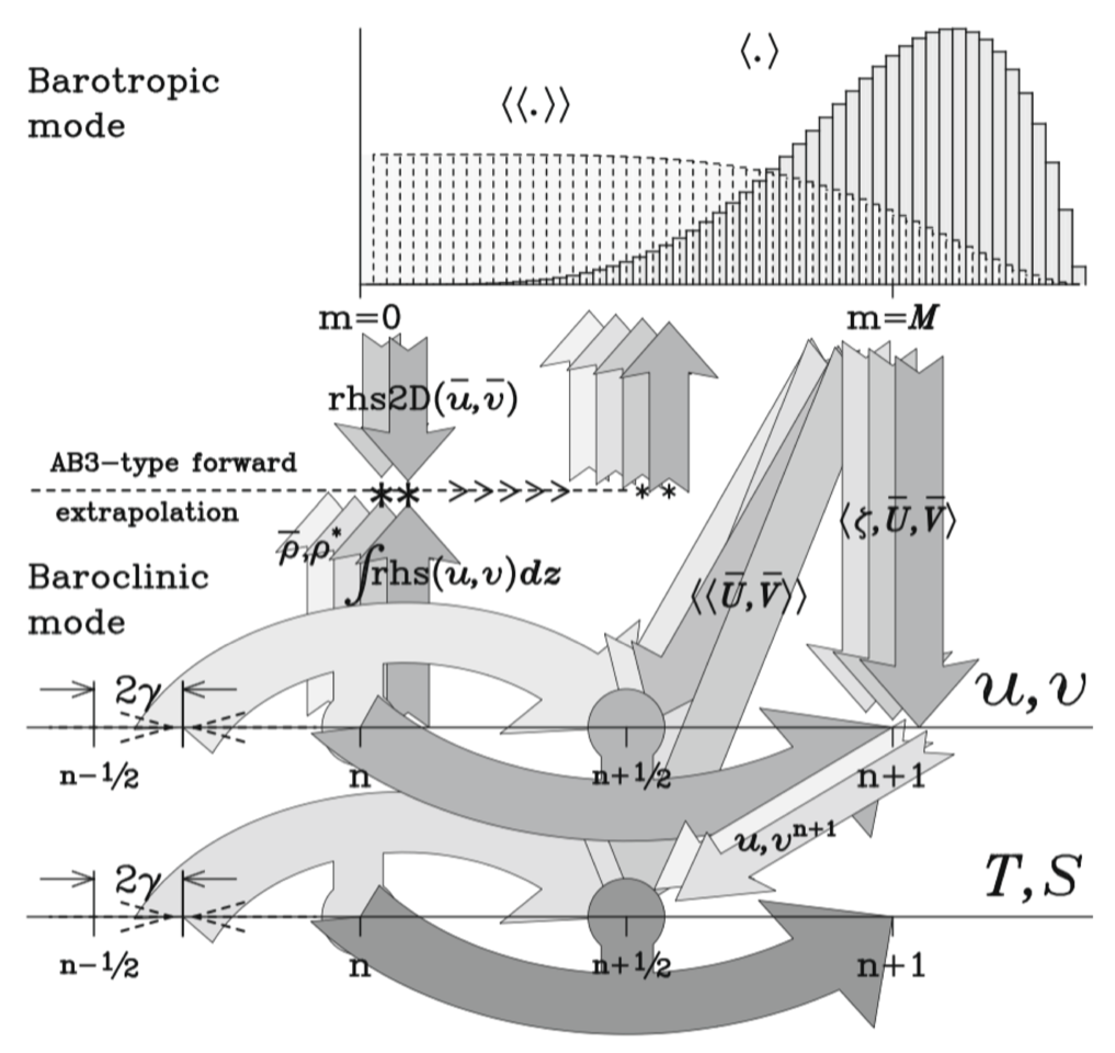
Fig: schematic view of the Croco predictor-corrector hydrostatic kernel#
General structure of the time-stepping:
call prestep3D_thread()    ! Predictor step for 3D momentum and tracers
call step2d_thread()       ! Barotropic mode
call step3D_uv_thread()   ! Corrector step for momentum
call step3D_t_thread()    ! Corrector step for tracers
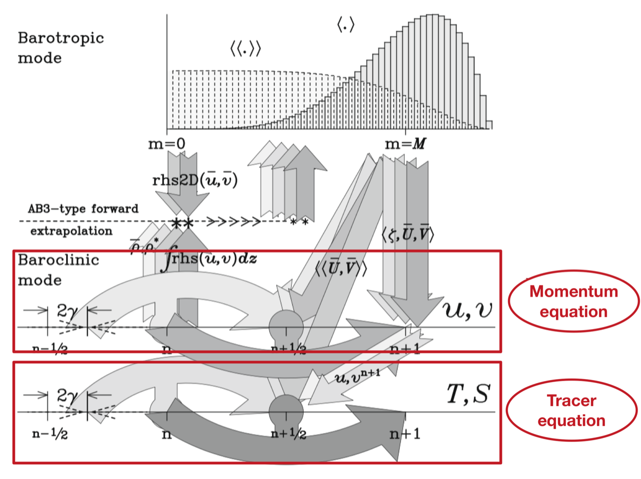
4.2.1. 3D momentum and tracers#
Predictor-corrector approach : Leapfrog (LF) predictor with 3rd-order Adams-Moulton (AM) interpolation (LFAM3 timestepping). This scheme is used to integrate 3D advection, the pressure gradient term, the continuity equation and the Coriolis term which are all contained in the \({\rm RHS}\) operator (the time tendencies).
For a given quantity \(q\) with \(q_t = {\rm RHS}(q)\) we can write
which can be rewritten in a compact way as used in the Croco code :
with \(\gamma = \frac{1}{6}\).
Physical parameterizations for vertical mixing, rotated diffusion and viscous/diffusion terms are computed once per time-step using an Euler step.
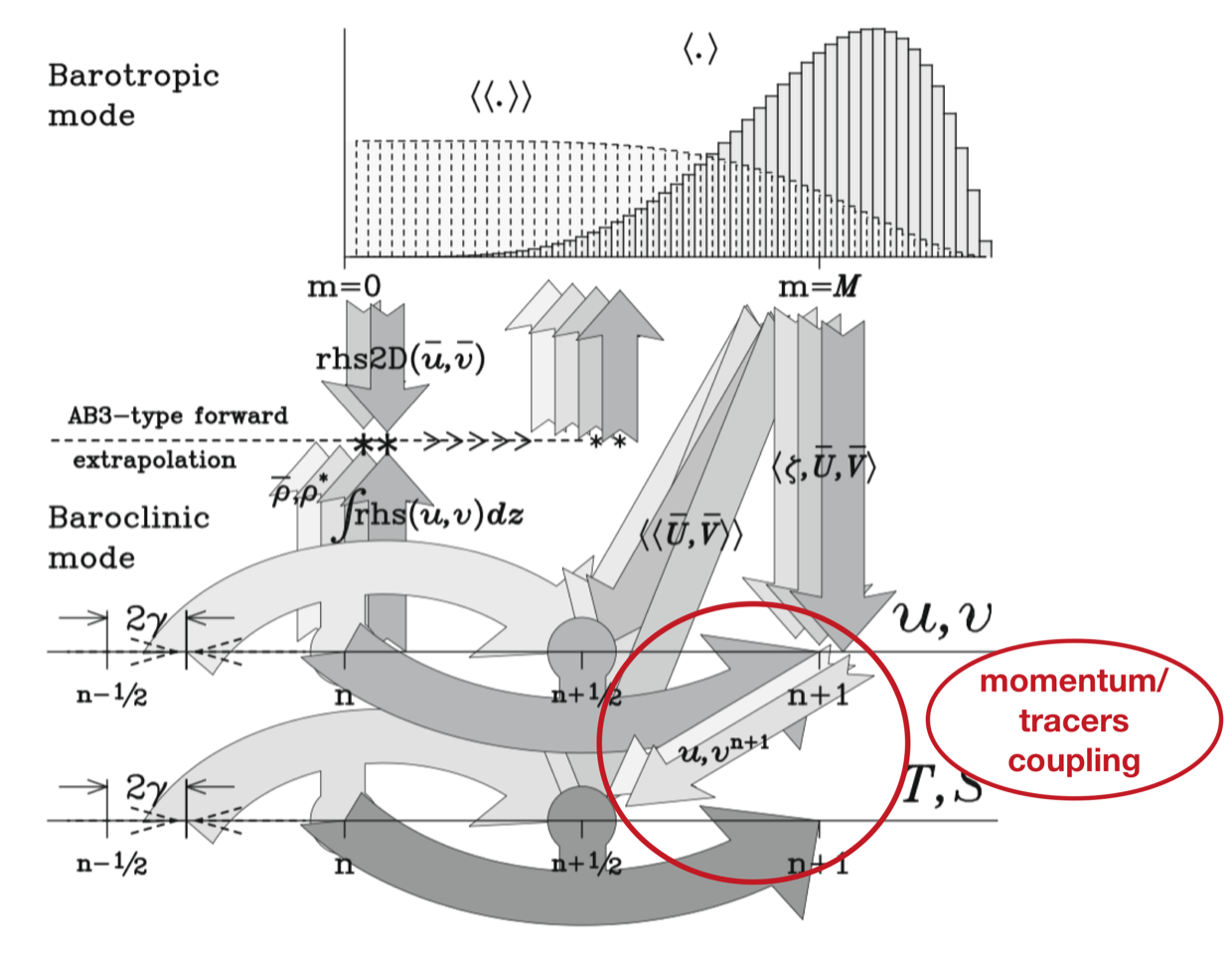
4.2.2. Tracers-momentum coupling#
The numerical integration of internal waves can be studied using the following subsystem of equations
Predictor step:
Corrector step:
Consequences:
3D-momentum integrated before the tracers in the corrector
2 evaluations of the pressure gradient per time-step
3 evaluations of the continuity equation per time-step
4.2.3. Barotropic mode#
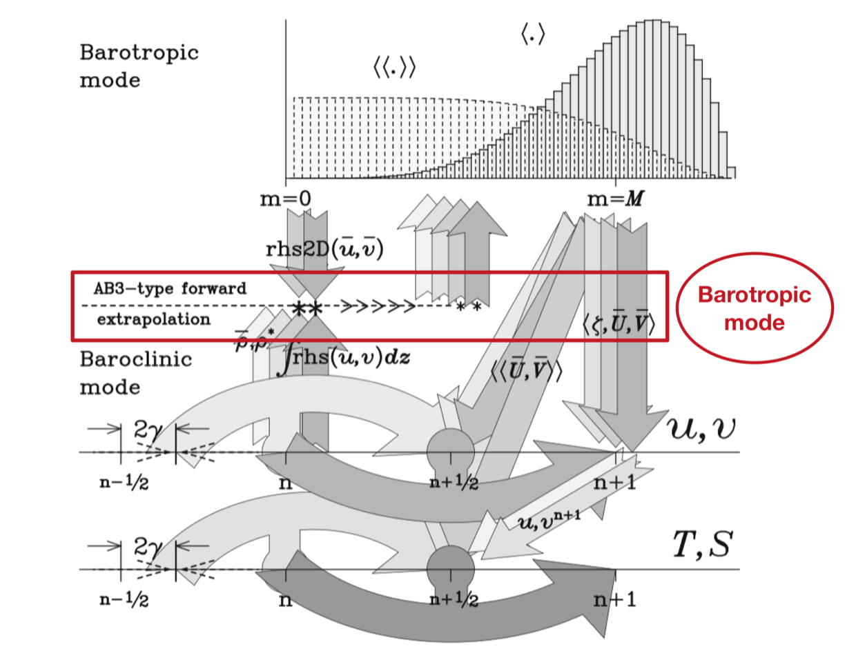
Generalized forward-backward (predictor-corrector)
AB3-type extrapolation
Integration of \(\zeta\)
AM4 interpolation
Integration of \(\bar{u}\)
where the parameter values are \((\beta,\gamma,\varepsilon)=(0.281105,0.088,0.013)\) except when the filter_none option is activated (see below).
4.2.4. Baroclinic-barotropic coupling#
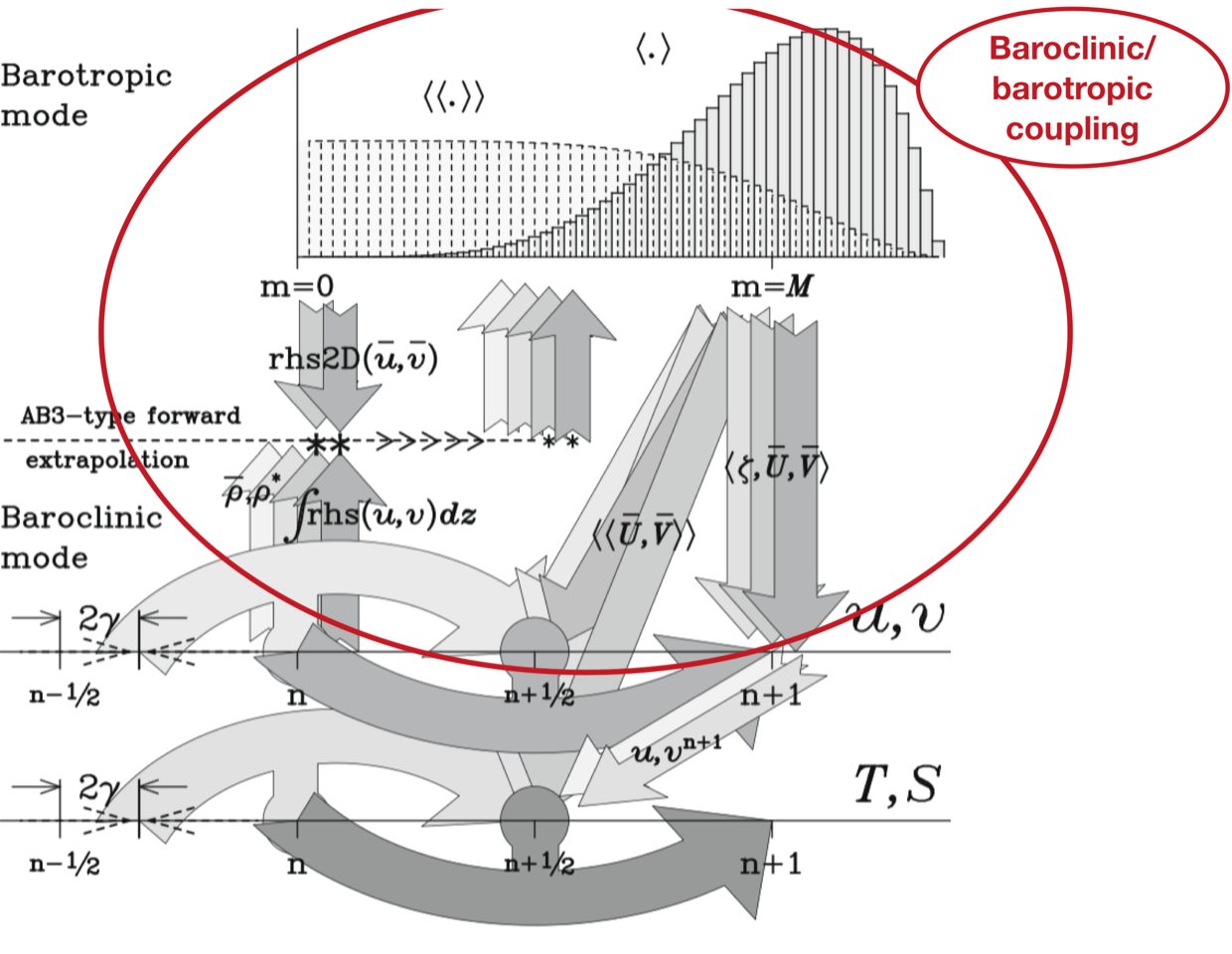
Slow forcing term of the barotrope by the barocline is extrapolated
4.2.4.1. M2_FILTER_POWER option#
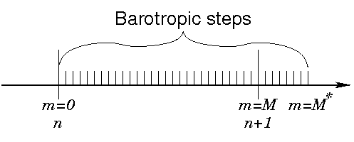
Barotropic integration from \(n\) to \(n+M^{*} \Delta \tau\) (\(M^{*} \le 1.5 M\))
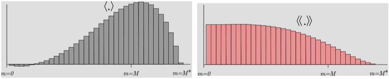
Because of predictor-corrector integration two barotropic filters are needed
\(\left< \zeta \right>^{n+1} \rightarrow \;\) update of the vertical grid
\(\left< U \right>^{n+1} \rightarrow \;\) correction of baroclinic velocities at time \(n+1\)
\(\left<\left< U \right>\right>^{n+\frac{1}{2}} \rightarrow \;\) correction of baroclinic velocities at time \(n+\frac{1}{2}\)
4.2.4.2. M2_FILTER_NONE option#
Motivation: averaging filters can lead to excessive dissipation in the barotropic mode
Objective: put the minimum amount of dissipation to stabilize the splitting
Diffusion is introduced within the barotropic time-stepping rather than averaging filters by adapting the parameters in the generalized forward-backward scheme
with \(\alpha_{\rm d} \approx 0.5\).
Remarks:
This option may require to increase \({\rm NDTFAST} = \varDelta t_{\rm 3D} / \varDelta t_{\rm 2D}\) because the stability constraint of the modified generalized forward-backward scheme is less than the one of the original generalized forward-backward scheme.
The filter_none approach is systematically more efficient than averaging filters
4.2.5. Stability constraints#
Barotropic mode (note that considering an Arakawa C-grid divides the theoretical stability limit by a factor of 2)
3D advection
where \(\alpha_{\rm adv}^x\), \(\alpha_{\rm adv}^y\), and \(\alpha_{\rm adv}^z\) are the Courant numbers in each direction and \(\beta = \alpha^\star_{\rm horiz} / \alpha^\star_{\rm vert}\) a coefficient arising from the fact that different advection schemes with different stability criteria may be used in the horizontal and vertical directions. Typical CFL values for \(\alpha^\star_{\rm horiz}\) and \(\alpha^\star_{\rm vert}\) with Croco time-stepping algorithm are
Advection scheme |
Max Courant number (\(\alpha^\star\)) |
|---|---|
C2 |
1.587 |
UP3 |
0.871 |
SPLINES |
0.916 |
C4 |
1.15 |
UP5 |
0.89 |
C6 |
1.00 |
Internal waves
where \(c_1\) the phase speed associated with the first (fastest) baroclinic mode.
Coriolis