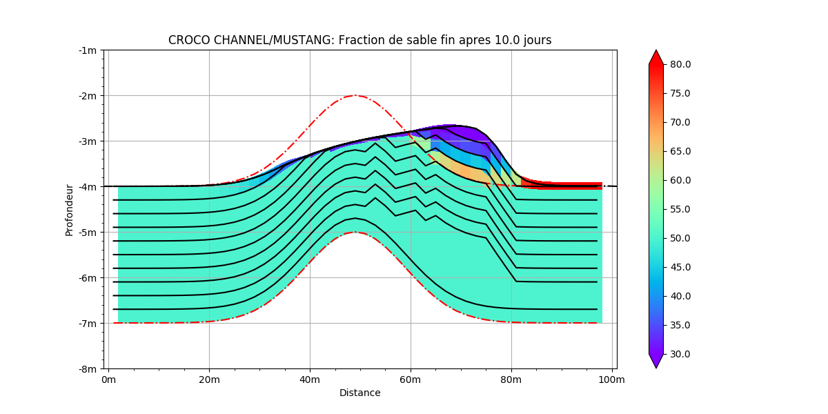
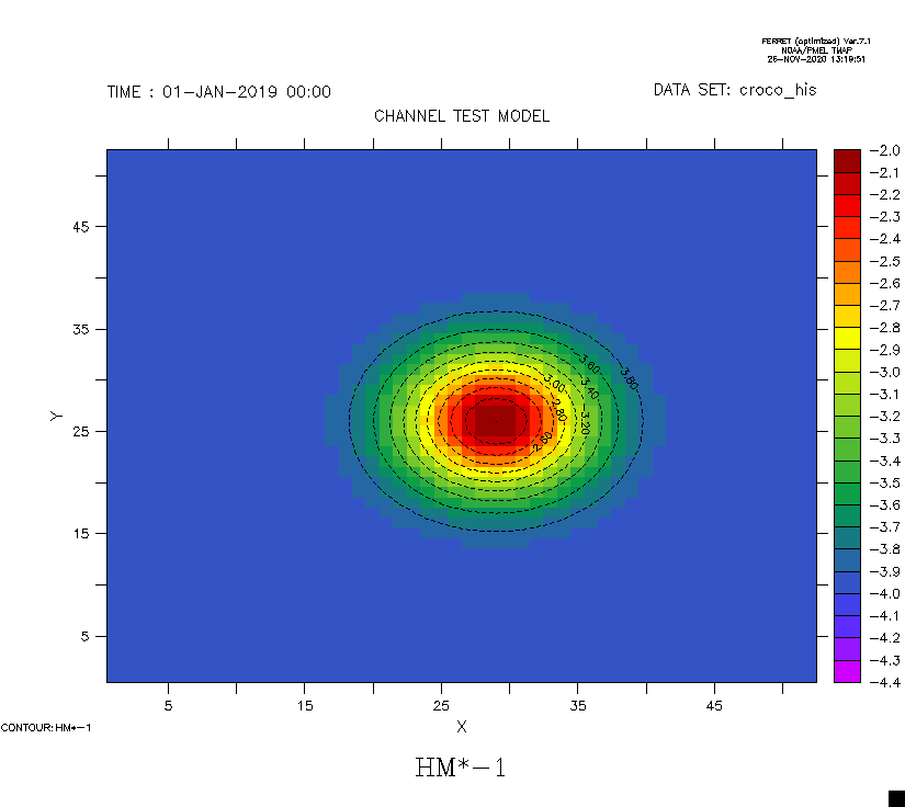
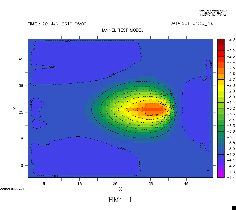
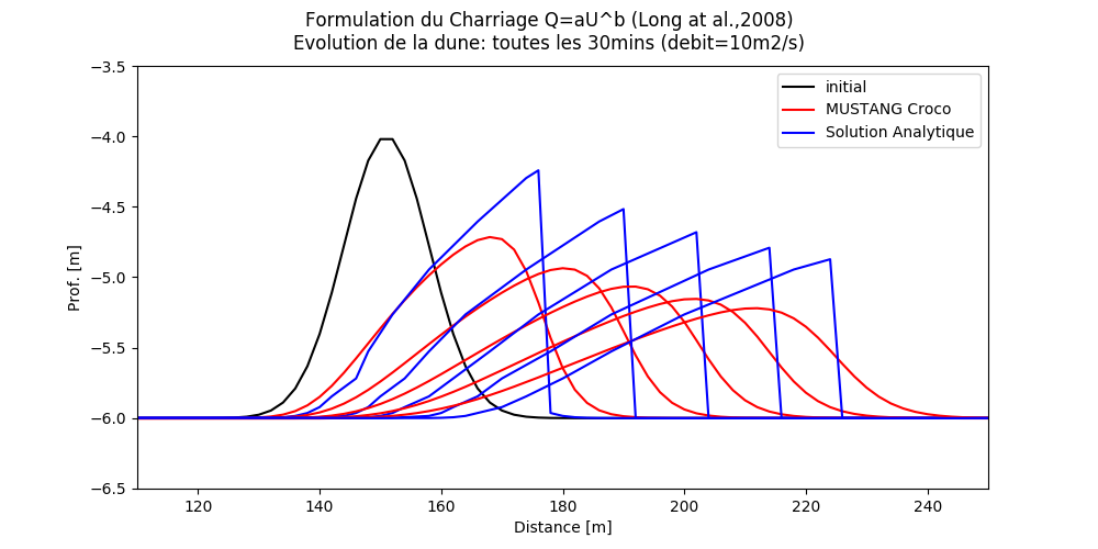
Adaptation of the DUNE case. Migration of a sand dune with an analytical bedload formulation that provides an analytical solution for the dune evolution (Long et al., 2008).
Wen Long, James T. Kirby, Zhiyu Shao, A numerical scheme for morphological bed level calculations, Coastal Engineering, Volume 55, Issue 2, 2008, Pages 167-180, https://doi.org/10.1016/j.coastaleng.2007.09.009
CPP options to add:
# define ANA_DUNE /* Analytical test case (Marieu) */# undef DUNE3D /* 3D example */
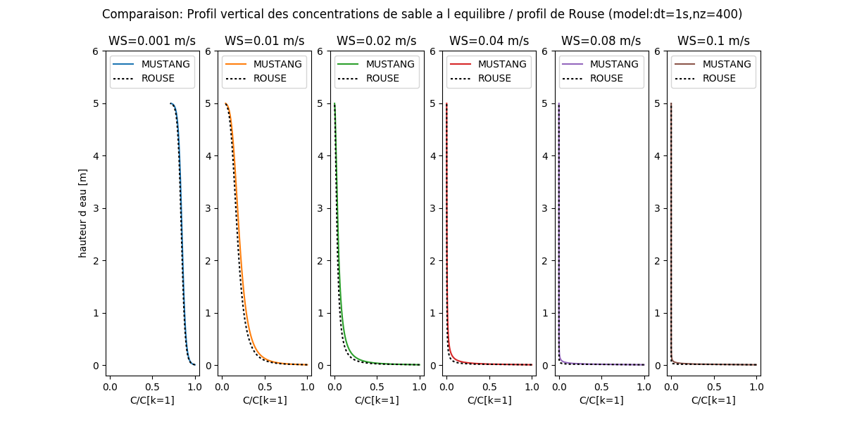
Comparison between suspended concentration and analytical Rouse profiles for 6 different settling velocities
SED_TOY/CONSOLID case :
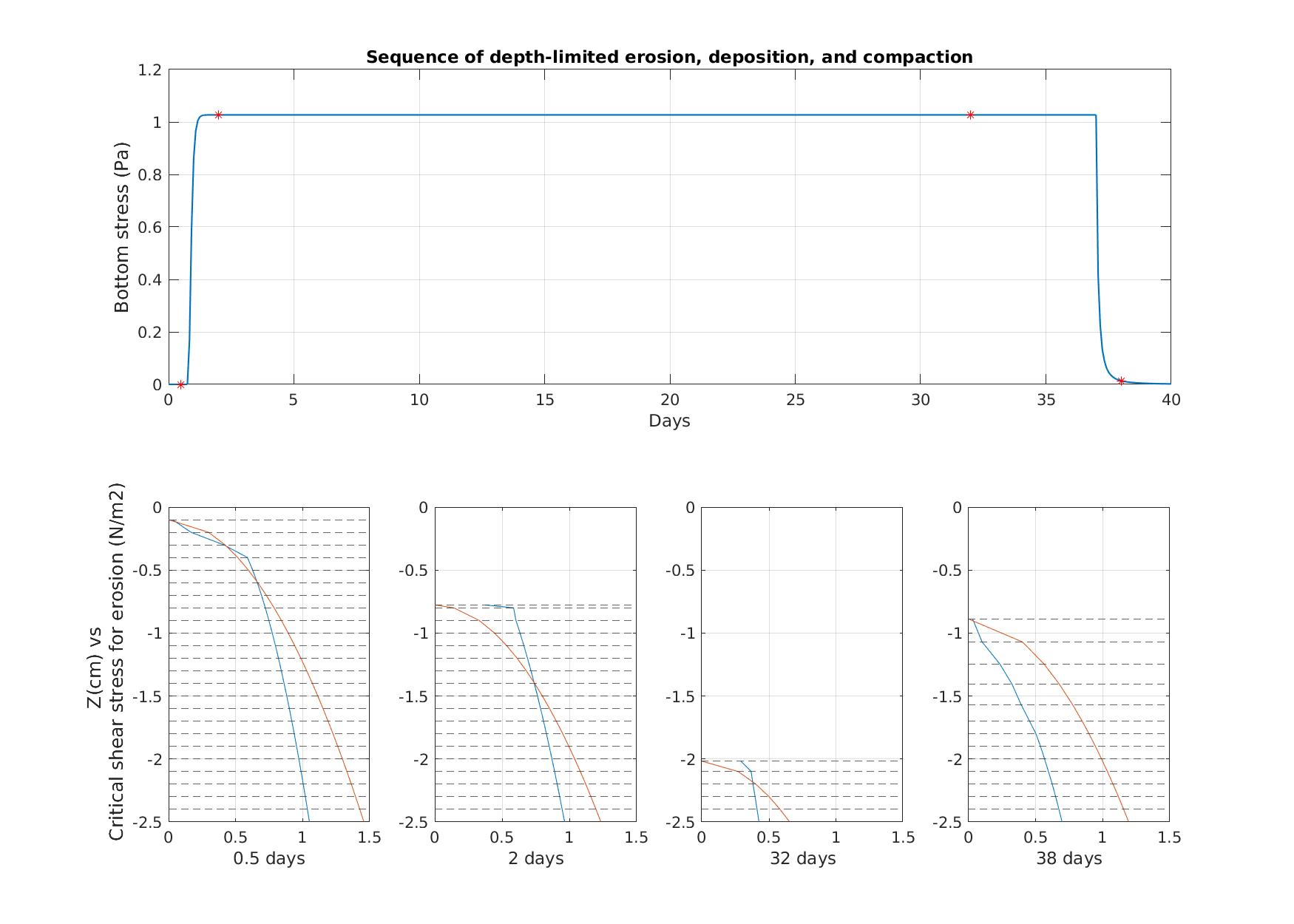
This 1DV test case exemplifies the sequence of depth-limited erosion, deposition, and compaction that characterizes the response of mixed and cohesive sediment in the model. From COAWST experiments, Cohesive and mixed sediment in the Regional Ocean Modeling System (ROMS v3.6) implemented in the Coupled Ocean–Atmosphere–Wave–Sediment Transport Modeling System (COAWST r1234) Sherwood et al., 2018, Geosci. Model Dev., 11, 1849–1871, 2018, https://doi.org/10.5194/gmd-11-1849-2018
2 sand classes and 2 mud classes, cohesive behaviour, up to 38 days :
Evolution of equilibrium bulk critical stress profile for erosion (red solid line) and the instantaneous profile of bulk critical stress for erosion (blue solid line)
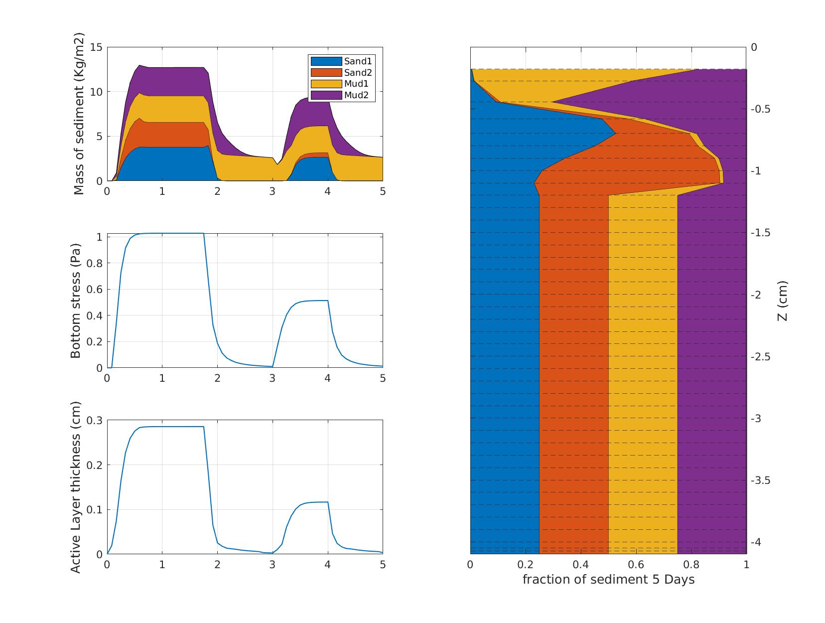
SED_TOY/RESUSP case :
This 1DV test case to demonstrate the evolution of stratigraphy caused by resuspension and subsequent settling of different class of sediment during time-dependent bottom shear stress events. From COAWST experiments, Cohesive and mixed sediment in the Regional Ocean Modeling System (ROMS v3.6) implemented in the Coupled Ocean–Atmosphere–Wave–Sediment Transport Modeling System (COAWST r1234) Sherwood et al., 2018, Geosci. Model Dev., 11, 1849–1871, 2018, https://doi.org/10.5194/gmd-11-1849-2018
2 sand classes and 2 mud classes, non cohesive behaviour:
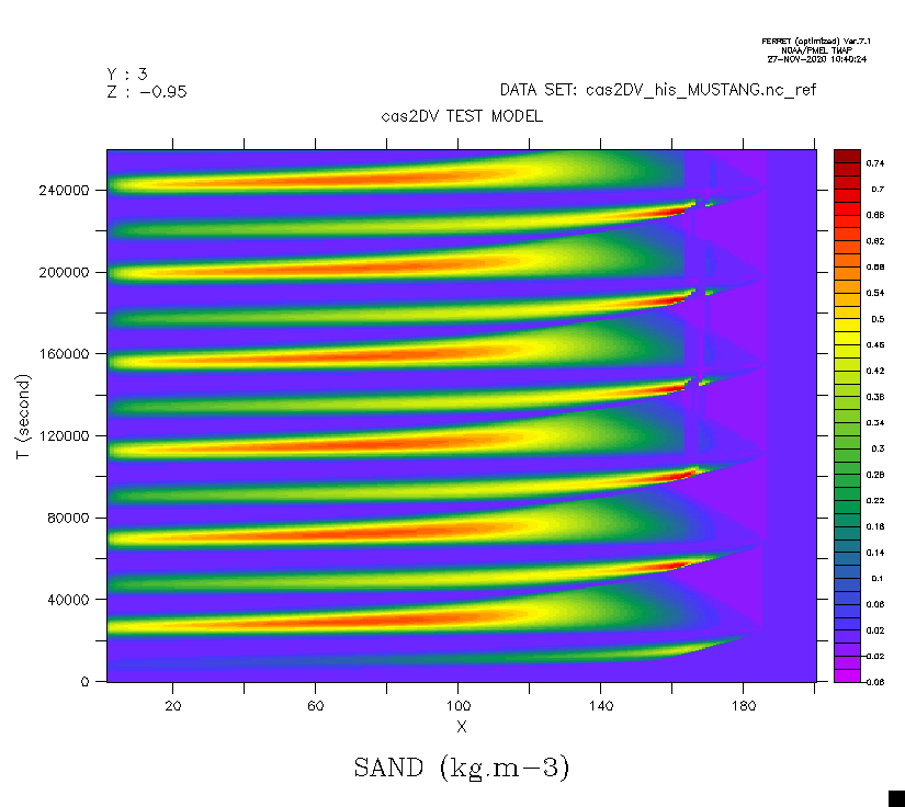
Bottom mud concentration evolution over several tidal cycles
FLOCMOD cases :
FLOCMOD 0D – comparison with laboratory experiments [#SED_TOY_FLOC_0D]
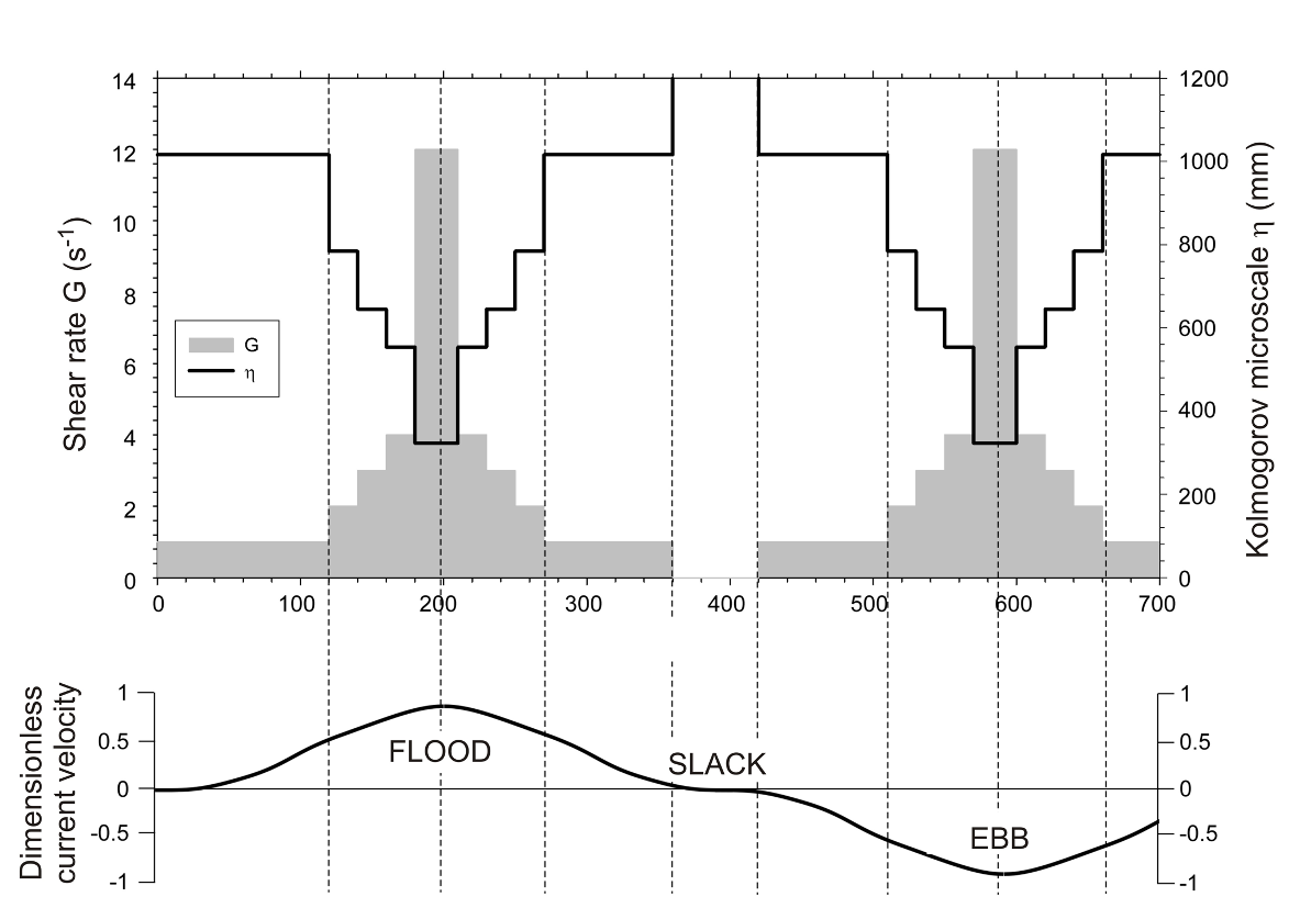
This test case simulates a laboratory experiment dedicated to flocculation experiments under controlled conditions (see Verney et al., 2011). Natural SPM were mixed in a jar and agitation was tuned to simulate turbulence variations during a tidal cycle. G values ranged from 1 s-1 (around slack periods) to 12 s-1 (during flood/ebb periods). Floc size were monitored using a CCD camera, and PSD were extracted from image processing routines.
This test case can be activated with the cppkey #SED_TOY_FLOC_0D. This test case has a 1DV structure but current is set to 0 (no advection, no diffusion), and settling is not allowed (Ws = 0 m.s-1 for all classes). Shear rate is imposed using experimental values in each vertical grid cell.
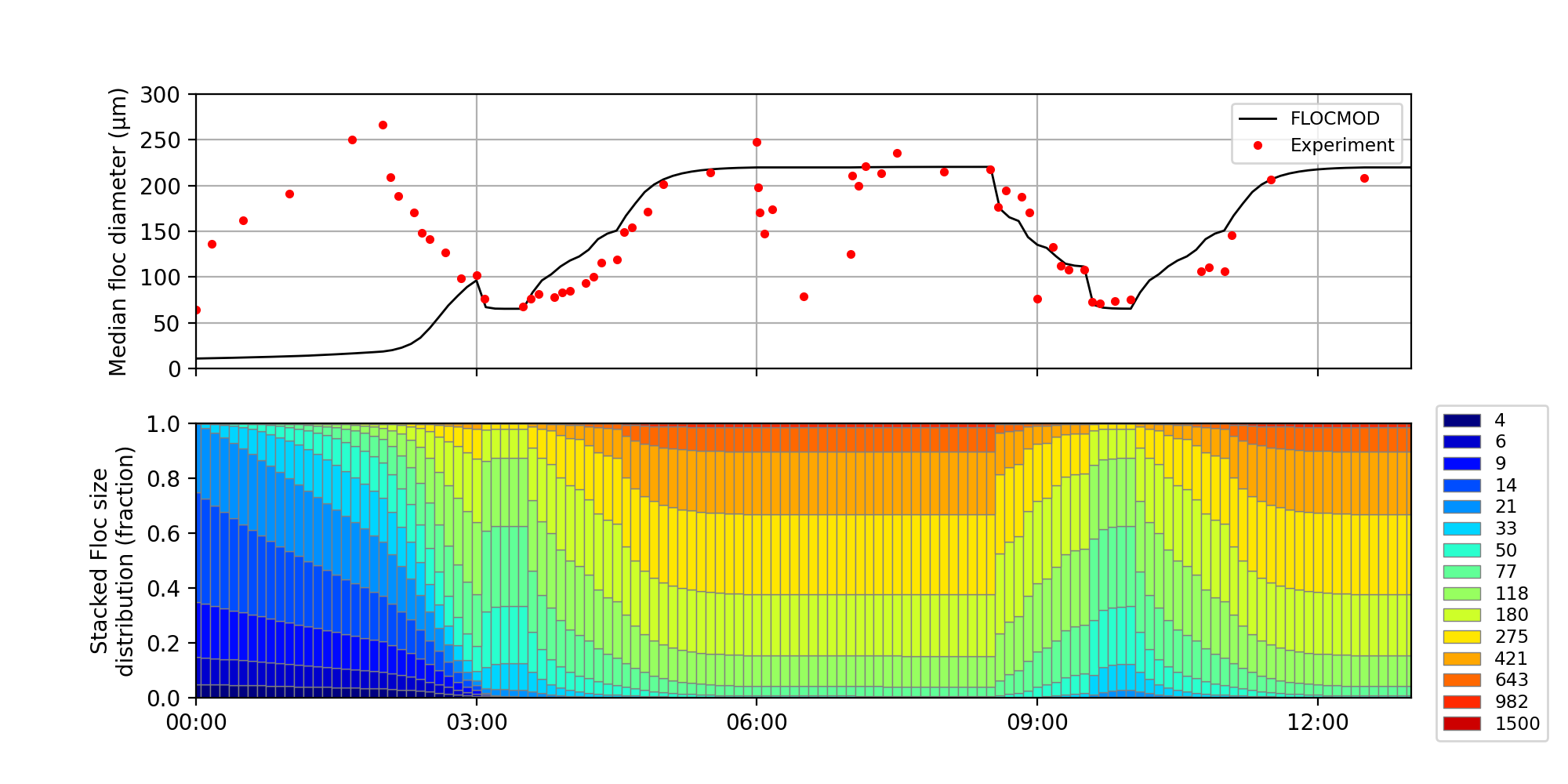
The initial concentration is set to 0.093 g.l-1 (experimental value) and the initial distribution is spread over the floc size classes lower than 50 \(\mu m\).
15 floc classes are used, logarithmically distributed from 4 \(\mu m\) to 1500 \(\mu m\). Primary particle size is set to 4 \(\mu m\) and nf = 1.9. CROCO time step is set to 2 s.
Shear aggregation and binary shear fragmentation only
FLOCMOD main parameters are : alpha = 0.43 and beta = 0.1.
Initial floc size distribution is far from the equilibrium, and FLOCMOD fails to reproduce the first flocculation period. After the first flood period, FLOCMOD and experimental results are in good agreement considering the D50. The settling phase observed in the experiment from 06:00 to 07:00 is not simulated in the 0D model.
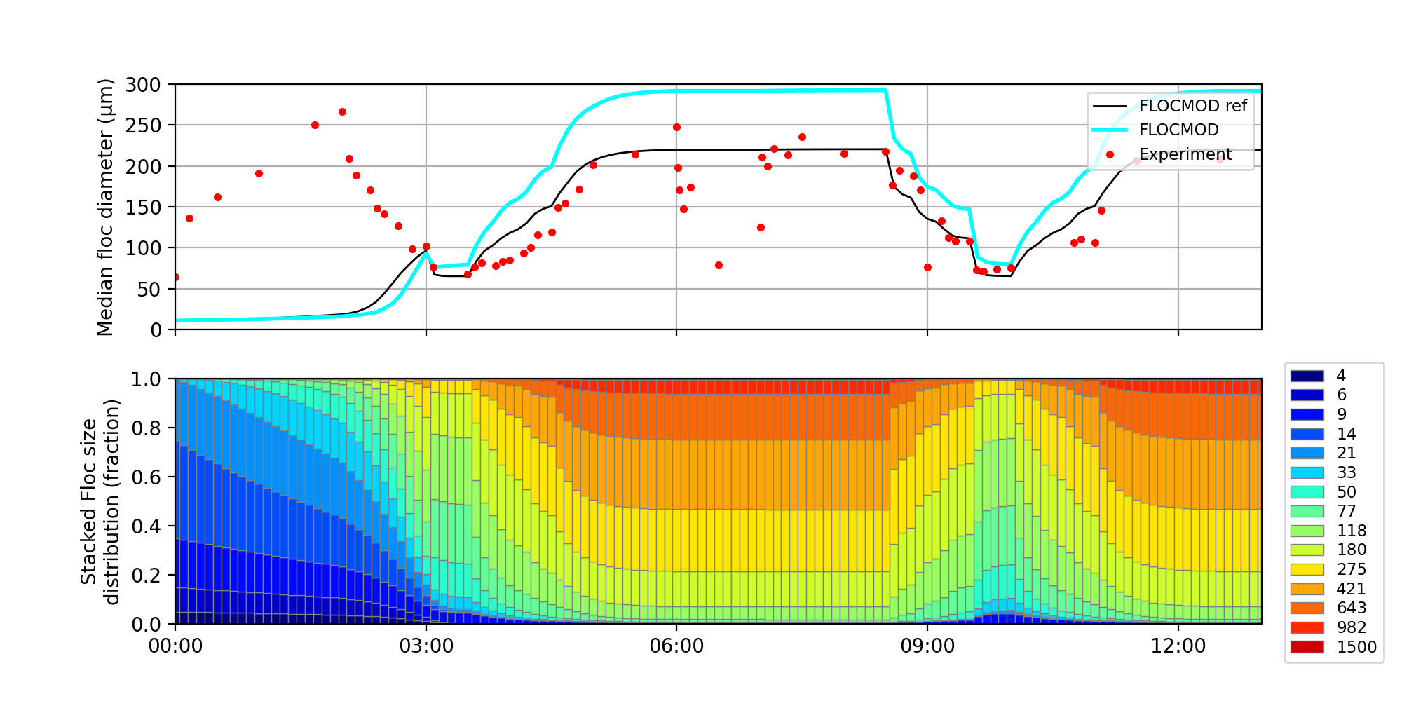
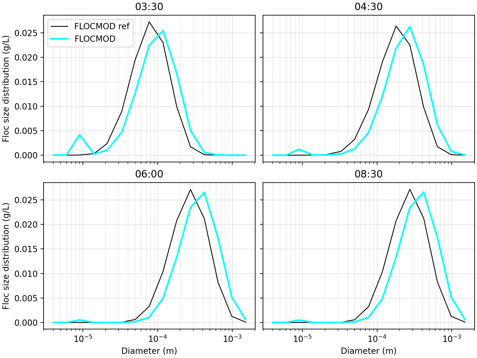
Shear aggregation, binary shear fragmentation and floc erosion
FLOCMOD main parameters are : alpha = 0.35 , beta = 0.1 , f_ero_frac = 0.4 and f_ero_iv = 3.
FLOCMOD reference is the shear aggregation/fragmentation test detailed above.
The median floc size dynamics is globally similar to the reference, however flocculation is more intense as part of shear fragmentation is attributed to floc erosion, hence flocs are less fragmented globally. We can also notice that erosion mode maintains a bimodal distribution, with a microfloc population (due to erosion) and macrofloc population varying in time with turbulence.
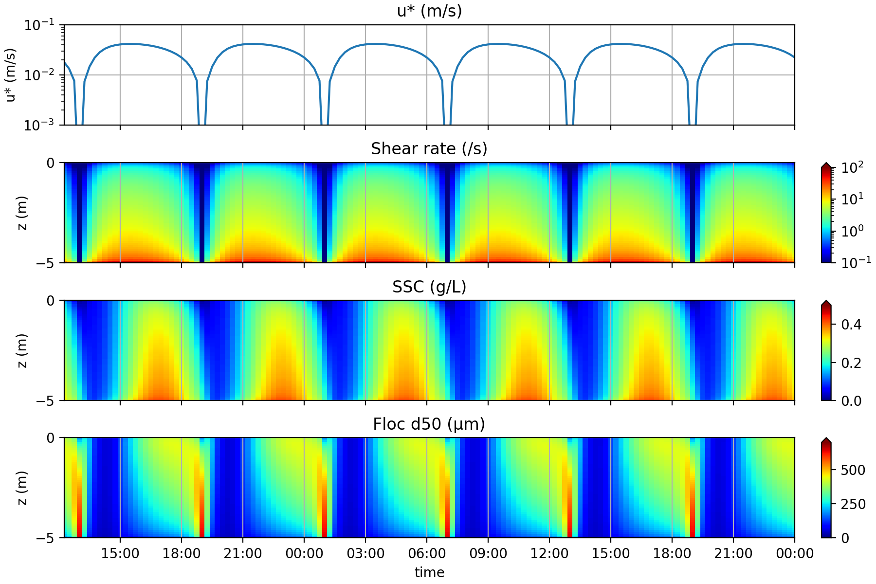
FLOCMOD 1DV [#SED_TOY_FLOC_1D]
This test case illustrates the vertical flocculation dynamics along a tidal cycle. 15 floc classes are used, logarithmically distributed from 4 \(\mu m\) to 1500 \(\mu m\). Primary particle size is set to 4 \(\mu m\) and nf = 1.9. CROCO time step is set to 10s.
CROCO main parameters are : h = 5 m, 50 vertical layers. A sinusoidal forcing is applied.
FLOCMOD main parameters are : alpha = 0.4 and beta = 0.2, including shear erosion and binary fragmentation: f_ero_frac = 0.5 and f_ero_iv = 4.
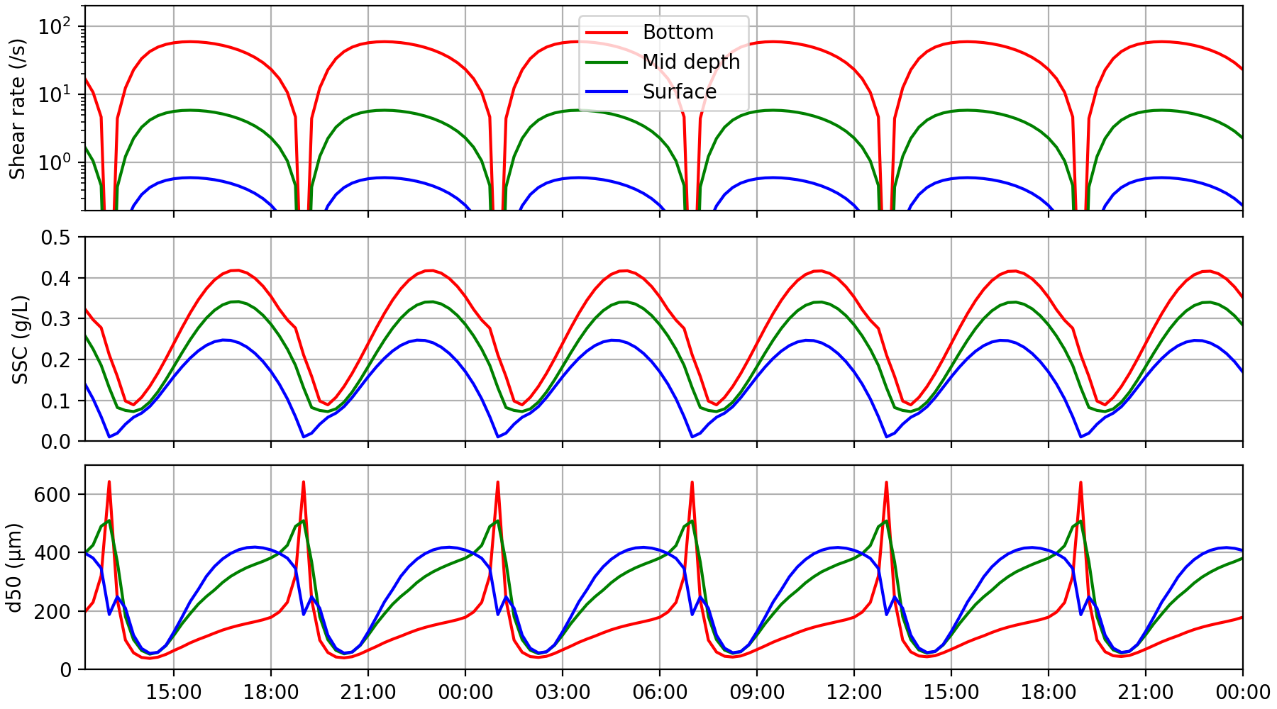
The shear rate varied from O(0.1 s-1) during slack to O(50 s-1) during max flood/ebb currents close to the bed. In the upper part of the water column, the shear rate is lower, and reaches up to O(1 s-1) during maximum current velocities.
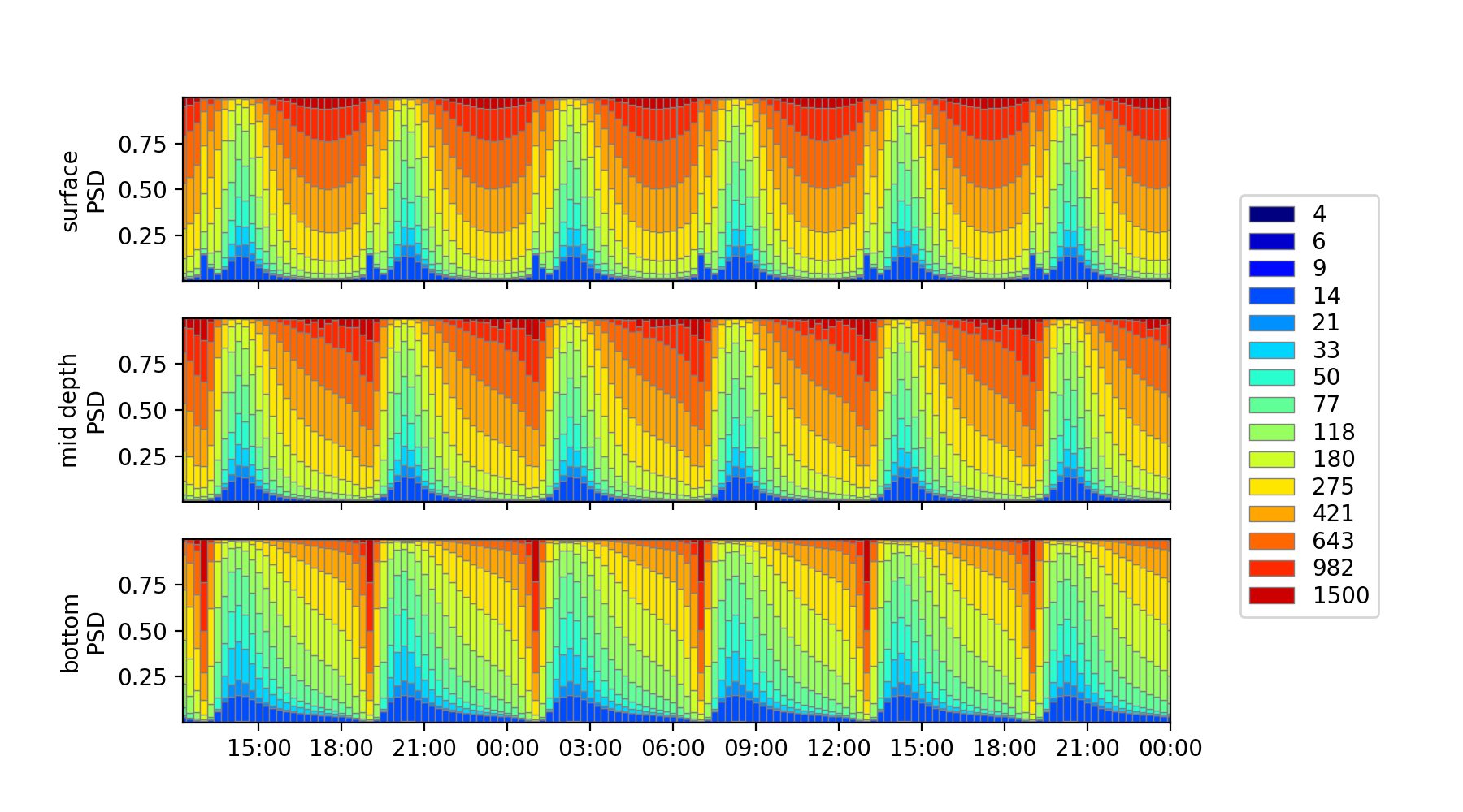
This tidal forcing induces resuspension during high shear stress periods, and SSC reaches up to 0.5 g/L close to the bed. Floc size distribution strongly varies along the tide, with the smallest floc sizes (\(~50 \mu m\)) close to the bed during maximum flood/ebb periods and the largest (\(~500 \mu m\)) during slack periods. We can note that flocculation starts earlier in the upper part of the water column, due to i) lower shear rate and ii) larger SSC values. Next flocs settle and accumulate close to the bed before settling in the sediment compartment.
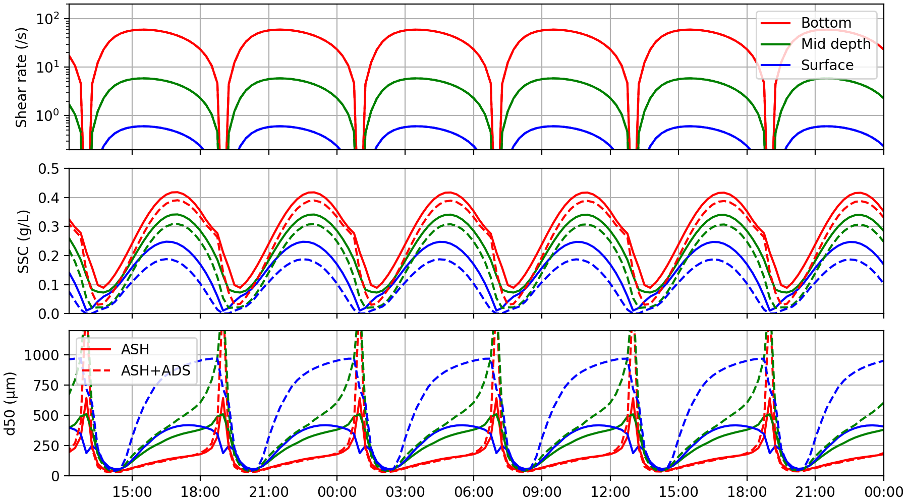
Adding differential settling aggregation
For this test, the same setup as above is used, and aggregation by differential settling is also activated (L_ADS=.TRUE.). Adding a complementary aggregation term (and a constant fragmentation term) induces a more intense flocculation, especially in the upper half of the water column, where the shear stress is less intense (D50 greater than 1mm). Close to the bed, the floc dynamics is similar to the reference, except during slack period where settling is dominant.
As a consequence, large floc sizes imply lower SSC especially in the upper part of the water column.
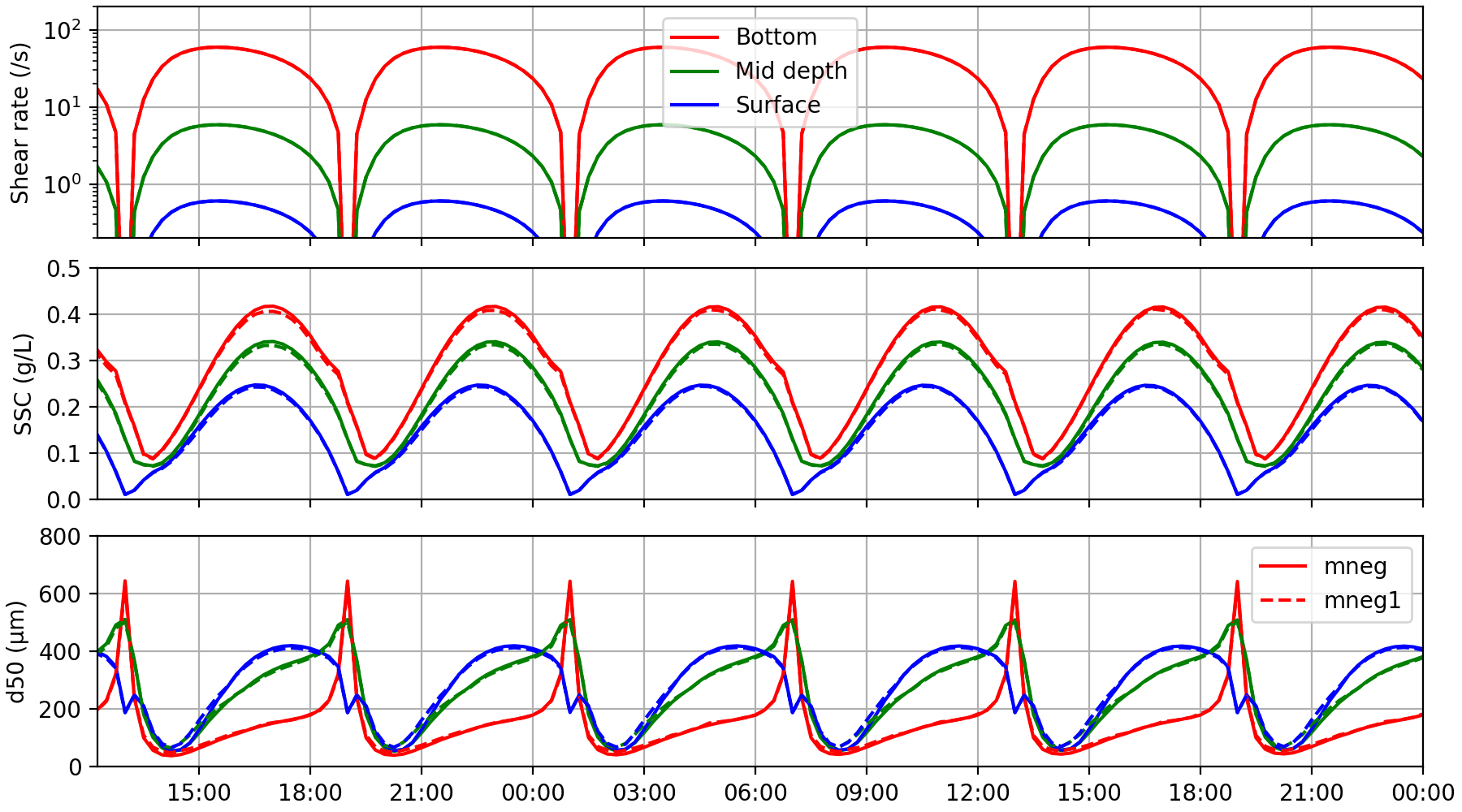
Adding “low negative mass option” mneg_param = 0.001 g/L.*
This test case is similar to the first 1DV test case (ADS not activated), except that low negative mass is “allowed” to limit the number of sub time steps. This means that when the total negative mass is below mneg_param, negative classes have their masses set to 0 and the remaining positive classes are proportionally lowered to ensure mass conservation.
Results are very similar both in term of SSC and floc D50, hence validating the possibility to use this option to improve computation time. For this 1DV configuration, activating this option decreased the computation time of about 30%.
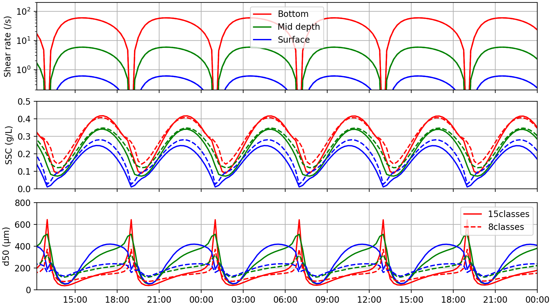
Passing from 15 classes to 8 classes
This last test concerns the number of classes to be used. The 15 original sediment classes are :
[4; 6; 9; 14; 21; 33; 50; 77; 118; 180; 275; 421; 643; 982; 1500] in \(\mu m\).
We run exactly the same configuration but with 8 classes :
[50; 77; 118; 180; 275; 421; 643; 982] in \(\mu m\).
In this case, flocculation is less intense, which can be explained by a less important numerical diffusion induced by small size classes (aggregating with the largest).
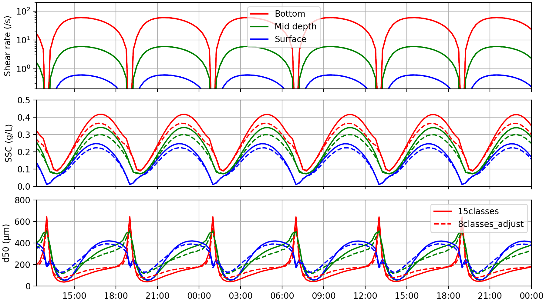
Very similar results compared with our reference (15 classes) can be obtained when tuning alpha (= 0.8) and f_ero_frac ( = 0.3).
Switching from 15 to 8 classes is crucial in term of computation time, saving up to 85% of computation time.