12.2.2. MUSTANG Sediment model
12.2.2.1. MUSTANG presentation
MUSTANG (MUd and Sand Tran ANSsport modelli NG) is a sediment module. Comparing to a pure hydrodynamical simulation, it adds variables relatives to sediment behavior such as sediment concentration in water and sediment bed evolution. This module has been developped by Le Hir et al, coupled with the hydrodynamic model SiAM. Then, it has continued to evolve, coupled with the parallelized MARS3D hydrodynamic model. It is now renamed MUSTANG (MUd and Sand TranSport modelliNG) and is available in the CROCO community model since release 1.2.
The module provides for the modeling of two types of sediment transport :
Bedload : sediment particles are set in motion from a certain critical tension. They move by staying close to the bottom
Suspension : sediment particles are suspended in the water column. They are transported in the water column as a passive tracer with a settling velocity through the advection-diffusion equation and eventually settle to the bottom.
MUSTANG module deals with various sediments classified into 3 types: GRAVEL, SAND and MUD. Gravels are transported only in bedload (no suspension). Sands can be transported by both types. Muds are transported only in suspension (no bedload).
From a sedimentary bottom consisting of a set of sedimentary facies, each of which is defined by a proportion of each of the classes, hydrosedimentary modeling consists of changing the proportions of each class of the sedimentary bottom as well as the thickness of the layers which constitute it, and therefore the bathymetry. It is then possible to inject the new bathymetry thus obtained into the hydrodynamic module (morphodynamic coupling).
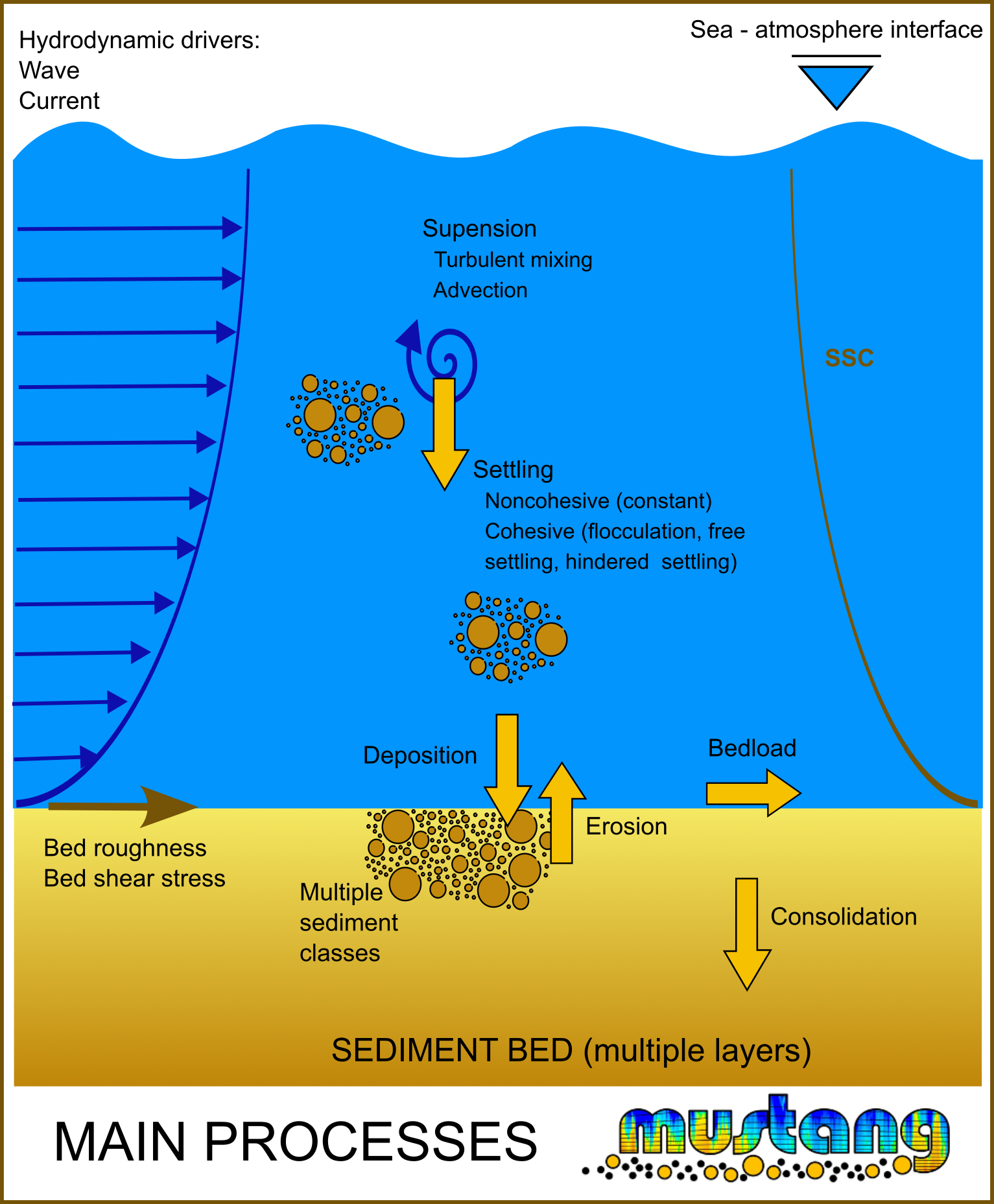
MUSTANG computes these evolutions by taking into account several processes such as settling, flocculation, erosion fluxes, deposit fluxes, consolidation (porosity) in sediment bed, bedload transport for non-cohesive sediment, morphodynamic…
There are 2 main options for this module :
one equivalent to the previous module “mixsed” (Le Hir et al, 2011) - default
one developped by Mengual & Le Hir (2018), which includes bedload processes (Rivier et al, 2017) - activated by cppkey #key_MUSTANG_V2
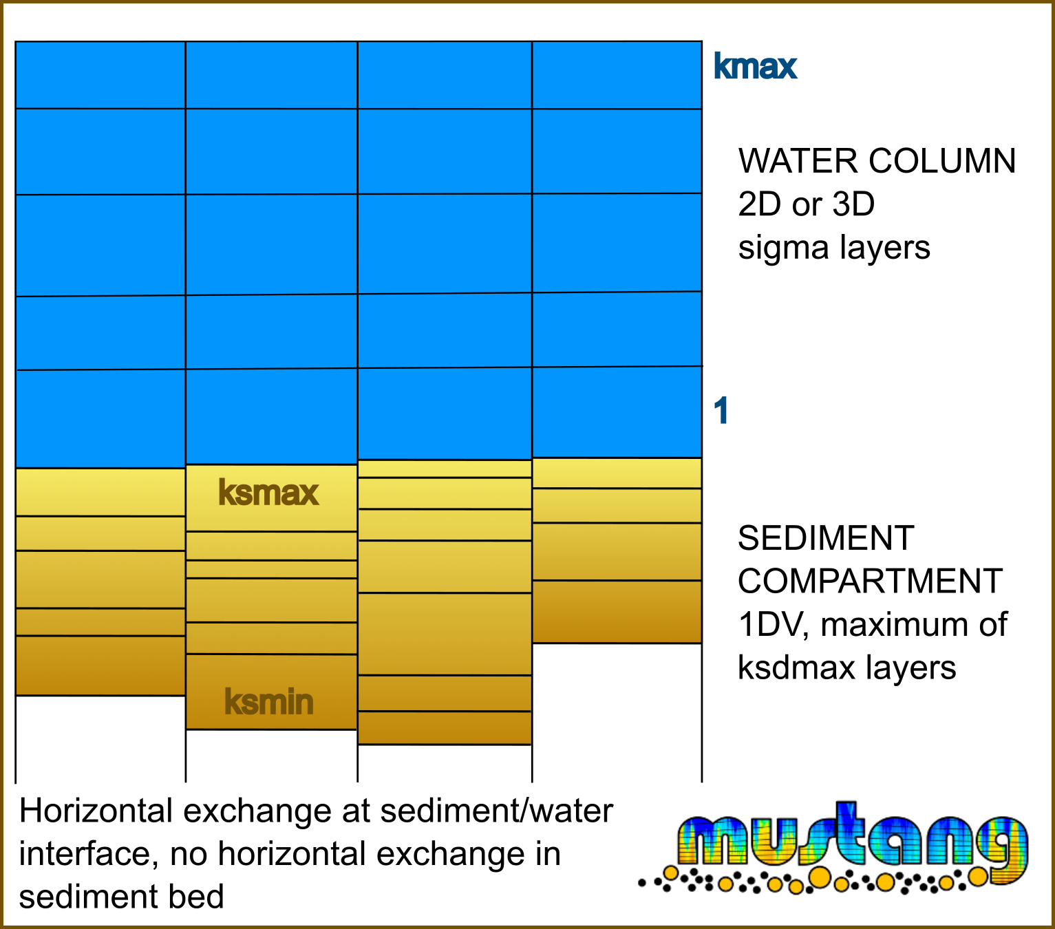
MUSTANG sediment compartment is 1DV in the sediment part, all exchanges between horizontal meshes, such as bedload, lateral erosion or sliding effect, are done at the interface between sediment and water.
MUSTANG consider 3 types of sediment but all features are not available for all type of sediment :
Type
Bedload transport
(if #key_MUSTANG_V2 & #key_MUSTANG_bedload)
Suspended load
Flocculation
(if #key_MUSTANG_flocmod)
MUD
NO
YES
YES
SAND
YES
YES
NO
GRAVEL
YES
NO
NO
Other substances can be defined via the susbstance module and can interact with sediment depending on their characteristics.
This documentation presents :
in MUSTANG user guide, input and output files format are detailed and available cppkeys are listed with a description of the effect of each key and a list of compatibility/incompatibility between keys
in MUSTANG technical documentation, a description of the insertion of MUSTANG calls in the CROCO temporal loop and a description of the modelisation of the main processes
in MUSTANG references the bibliography
12.2.2.2. MUSTANG user guide
MUSTANG module can not be used alone, it needed an hydrodynamic model and the substance module.
In this documentation, the hydrodynamic model is CROCO. Hydrodynamic parametrization will not be detailed here, please refer to hydrodynamic module documentation.
To use MUSTANG in CROCO you will need to :
define appropriate cppkeys in cppdefs.h. To activate MUSTANG within CROCO environment, the MUSTANG and SUBSTANCE cppkeys must be defined. To activate certains processes other cppkeys must be defined (see available cppkeys)
define MUSTANG and SUBSTANCE files in CROCO input file croco.in, these file contains MUSTANG parameters and SUBSTANCE characteristics (see MUSTANG namelist and SUBSTANCE namelist)
define appropriate dimensions in param.h file
depending on the options you choose via your cppkeys and input file (MUSTANG namelist and SUBSTANCE namelist), you will have to define other input file such as initialization file, wave file, source with solid discharge file
Then you can compile and run CROCO as any other CROCO run.
Note
MUSTANG is controlled through both CPP keys and input files. For some processes it is needed to activate the options through a CPP key, and also through a flag (true or false) in the input files
12.2.2.2.1. Input file : croco.in
The name and location of the MUSTANG and SUBSTANCE input files are defined in CROCO input file croco.in as follow:
sediments_mustang: input file
               MUSTANG_NAMELIST/parasubstance.txt
               MUSTANG_NAMELIST/paraMUSTANG.txt
In this example, the files are located in MUSTANG_NAMELIST directory but they could be placed in any directory. Therefore, example and test cases namelists could be found in MUSTANG_NAMELIST directory in MUSTANG source directory.
In particular, in MUSTANG_NAMELIST directory (relative path from the current directory where croco executable is), a file paraMUSTANG_default.txt contains all default values used, if the user does not specify a parameter in the namelist file, the default value in MUSTANG_NAMELIST/paraMUSTANG_default.txt is used.
There is no default file for susbstance but a full example is given in MUSTANG_NAMELIST directory in MUSTANG source directory.
12.2.2.2.2. Input file : param.h
Before the code compilation, the following dimensions must be defined in the param.h file to use SUBSTANCE and MUSTANG :
ksdmin and ksdmax: integers corresponding to the layers of sediment (sediment variables are allocated with ksdim:ksdmax dimension)
ntrc_subs: number of substance corresponding to a tracer (advected)
ntfix: number of fixed substance (not advected)
ntrc_substot: total number of substance (= ntrc_subs + ntfix)
If these dimensions are modified, the code must be compiled again.
12.2.2.2.3. Input file : Substance namelist
Substance module allow to define 8 different types of substance with different behavior. Sediments are defined as MUD, SAND or GRAVEL.
Substance input file contains at least 5 namelists and at most 9 namelists depending on the cppkeys MUSTANG and key_benthic :
nmlnbvar : number of each type of substance to be defined (other than T (temperature) & S (salinity))
nmlpartnc : characterization of Non Constitutive Particulate subtances
nmlpartsorb : characterization of particulate susbtances sorbed on an other particule
nmlvardiss : characterization of dissolved susbtances
nmlvarfix :characterization of fixed susbtances (not advected)
nmlgravels (if MUSTANG only) : characterization of GRAVEL substances
nmlsands (if MUSTANG only) : characterization of SAND substances
nnmlmuds (if MUSTANG only) : characterization of MUD substances
nmlvarbent (if key_benthic only) : characterization of benthic substances
Each namelist is described bellow with the description of each parameter.
&nmlnbvar namelist:
nv_dis : number of dissolved susbtances
nv_ncp: number of Non Constitutive Particulate subtances, like for example trace metals, bacteria, nitrogen, organic matter.
nv_fix : number of fixed susbtances (not advected)
nv_bent : number of benthic susbtances
nv_grav : number of Constitutive susbtances type GRAVELS (only if cppkey MUSTANG)
nv_sand : number of Constitutive susbtances type SAND (only if cppkey MUSTANG)
nv_mud : number of Constitutive susbtances type MUD (only if cppkey MUSTANG)
nv_sorb : number of particulate susbtances sorbed on an other particule
Note
If MUSTANG cpp key is not defined, nv_grav, nv_sand and nv_mud are not read and must not be present
&nmlgravels namelist: each parameter is a vector of length nv_grav
name_var_n() : name of variable
long_name_var_n() : long name of variable
standard_name_var_n() : standard name of variable
unit_var_n() : string, unit of concentration of variable
flx_atm_n() : uniform atmospherical deposition (unit/m2/s)
cv_rain_n() : concentration in rainwater (kg/m3 of water)
cini_wat_n() : initial concentration in water column (kg/m3)
cini_air_n() : initial concentration in air
l_out_subs_n() : saving in output file if TRUE
init_cv_name_n() : name of substance read from initial condition file
obc_cv_name_n() : name of substance read from obc file
cini_sed_n() : initial fraction in the seafloor (only if cppkey MUSTANG)
tocd_n() : critical stress of deposition (N/m2) (only if cppkey MUSTANG)
ros_n() : density of particle (kg/m3) (only if cppkey MUSTANG)
l_bedload_n() : allow bedload transport if true (only if cppkey MUSTANG and key_MUSTANG_V2 and key_MUSTANG_bedload)
diam_n() : diameter of particles (m)
Note
If nv_grav = 0 this namelist is not read.
&nmlsands namelist: each parameter is a vector of length nv_sand
name_var_n() : name of variable
long_name_var_n() : long name of variable
standard_name_var_n() : standard name of variable
unit_var_n() : string, unit of concentration of variable
flx_atm_n() : uniform atmospherical deposition (unit/m2/s)
cv_rain_n() : concentration in rainwater (kg/m3 of water)
cini_wat_n() : initial concentration in water column (kg/m3)
cini_air_n() : initial concentration in air
l_out_subs_n() : saving in output file if TRUE
init_cv_name_n() : name of substance read from initial condition file
obc_cv_name_n() : name of substance read from obc file
cini_sed_n() : initial fraction in the seafloor (only if cppkey MUSTANG)
tocd_n() : critical stress of deposition (N/m2) (only if cppkey MUSTANG)
ros_n() : density of particle (kg/m3) (only if cppkey MUSTANG)
l_bedload_n() : allow bedload transport if true (only if cppkey MUSTANG and key_MUSTANG_V2 and key_MUSTANG_bedload)
diam_n() : diameter of particles (m)
l_sand2D() : treat sand variable as 2D variable if true (used only if key_sand2D, see Treatment of high settling velocities : SAND variables)
l_outsandrouse() : if true, use a reconstitution of a ROUSE profil for output in water column (used only if key_sand2D and l_sand2D is TRUE for this variable, see Treatment of high settling velocities : SAND variables)
Note
If nv_sand = 0 this namelist is not read.
Warning
If you have several sands in your simulation : start with the coarser sands and continue more and more finely
&nmlmuds namelist: each parameter is a vector of length nv_mud
name_var_n() : name of variable
long_name_var_n() : long name of variable
standard_name_var_n() : standard name of variable
unit_var_n() : string, unit of concentration of variable
flx_atm_n() : uniform atmospherical deposition (unit/m2/s)
cv_rain_n() : concentration in rainwater (kg/m3 of water)
cini_wat_n() : initial concentration in water column (kg/m3)
cini_air_n() : initial concentration in air
l_out_subs_n() : saving in output file if TRUE
init_cv_name_n() : name of substance read from initial condition file
obc_cv_name_n() : name of substance read from obc file
cini_sed_n() : initial fraction in the seafloor (only if cppkey MUSTANG)
tocd_n() : critical stress of deposition (N/m2) (only if cppkey MUSTANG)
ros_n() : density of particle (kg/m3) (only if cppkey MUSTANG)
cobc_wat_n() : boundaries uniform and constant concentration (kg/m3)
ws_free_opt_n() : integer, choice of free settling formulation : 0 constant, 1 Van Leussen, 2 Winterwerp, 3 Wolanski (see Settling velocity)
ws_free_min_n() : minimum setling velocity (m/s) (see Settling velocity)
ws_free_max_n() : maximum setling velocity (m/s) (see Settling velocity)
ws_free_para_n(1:4,num substance) : 4 additional parameters (see Settling velocity)
ws_hind_opt_n() : choice of hindered settling formulation : 0 no hindered settling, 1 Scott, 2 Winterwerp, 3 Wolanski (see Settling velocity)
ws_hind_para_n(1:2,num substance) : 2 additional parameters (see Settling velocity)
diam_n() : diameter of particles (m) (used only if #key_mustang_flocmod is activated see FLOCMOD )
Note
If nv_mud = 0 this namelist is not read.
&nmlpartnc namelist: each parameter is a vector of length nv_ncp
name_var_n() : name of variable
long_name_var_n() : long name of variable
standard_name_var_n() : standard name of variable
unit_var_n() : string, unit of concentration of variable
flx_atm_n() : uniform atmospherical deposition (unit/m2/s)
cv_rain_n() : concentration in rainwater (kg/m3 of water)
cini_wat_n() : initial concentration in water column (kg/m3)
cini_air_n() : initial concentration in air
l_out_subs_n() : saving in output file if TRUE
init_cv_name_n() : name of substance read from initial condition file
obc_cv_name_n() : name of substance read from obc file
cini_sed_n() : initial concentration in sediment (quantity/kg of dry sediment) (only if cppkey MUSTANG)
tocd_n() : critical stress of deposition (N/m2) (only if cppkey MUSTANG)
ros_n() : density of particle (kg/m3) (only if cppkey MUSTANG)
cobc_wat_n() : boundaries uniform and constant concentration (kg/m3)
ws_free_opt_n() : integer, choice of free settling formulation : 0 constant, 1 Van Leussen, 2 Winterwerp, 3 Wolanski (see Settling velocity)
ws_free_min_n() : minimum setling velocity (m/s) (see Settling velocity)
ws_free_max_n() : maximum setling velocity (m/s) (see Settling velocity)
ws_free_para_n(1:4,num substance) : 4 additional parameters (see Settling velocity)
ws_hind_opt_n() : choice of hindered settling formulation : 0 no hindered settling, 1 Scott, 2 Winterwerp, 3 Wolanski (see Settling velocity)
ws_hind_para_n(1:2,num substance) : 2 additional parameters (see Settling velocity)
Note
If nv_ncp = 0 this namelist is not read.
If MUSTANG cpp key is not defined, cini_sed_n, tocd_n, ros_n, ws_free_opt_n, ws_free_para_n, ws_hind_opt_n, ws_hind_para_n are not read and must not be present
&nmlpartsorb namelist: each parameter is a vector of length nv_sorb
name_var_n() : name of variable
long_name_var_n() : long name of variable
standard_name_var_n() : standard name of variable
unit_var_n() : string, unit of concentration of variable
flx_atm_n() : uniform atmospherical deposition (unit/m2/s)
cv_rain_n() : concentration in rainwater (kg/m3 of water)
cini_wat_n() : initial concentration in water column (kg/m3)
cini_air_n() : initial concentration in air
l_out_subs_n() : saving in output file if TRUE
init_cv_name_n() : name of substance read from initial condition file
obc_cv_name_n() : name of substance read from obc file
cini_sed_n() : initial concentration in sediment (quantity/kg of dry sediment) (only if cppkey MUSTANG)
cobc_wat_n() : boundaries uniform and constant concentration (kg/m3)
name_varpc_assoc_n() : name of associated particulate substance on which this substance is sorbed
Note
If nv_sorb = 0 this namelist is not read.
If MUSTANG cpp key is not defined, cini_sed_n is not read and must not be present
&nmlvardiss namelist: each parameter is a vector of length nv_dis
name_var_n() : name of variable
long_name_var_n() : long name of variable
standard_name_var_n() : standard name of variable
unit_var_n() : string, unit of concentration of variable
flx_atm_n() : uniform atmospherical deposition (unit/m2/s)
cv_rain_n() : concentration in rainwater (kg/m3 of water)
cini_wat_n() : initial concentration in water column (kg/m3)
cini_air_n() : initial concentration in air
l_out_subs_n() : saving in output file if TRUE
init_cv_name_n() : name of substance read from initial condition file
obc_cv_name_n() : name of substance read from obc file
cini_sed_n() : initial concentration in sediment (quantity/kg of dry sediment) (only if cppkey MUSTANG)
cobc_wat_n() : boundaries uniform and constant concentration (kg/m3)
Note
If nv_dis = 0 this namelist is not read.
If MUSTANG cpp key is not defined, cini_sed_n is not read and must not be present
&nmlvarfix namelist: each parameter is a vector of length nv_fix
name_var_fix() : name of variable
long_name_var_fix() : long name of variable
standard_name_var_fix() : standard name of variable
unit_var_fix() : string, unit of concentration of variable
cini_wat_fix() : initial concentration in water column (kg/m3)
l_out_subs_fix() : saving in output file if TRUE
init_cv_name_fix() : name of substance read from initial condition file
Note
If nv_fix = 0 this namelist is not read.
&nmlvarbent namelist: each parameter is a vector of length nv_bent
name_var_bent() : name of variable
long_name_var_bent() : long name of variable
standard_name_var_bent() : standard name of variable
unit_var_bent() : string, unit of concentration of variable
cini_bent() : initial concentration
l_out_subs_bent() : saving in output file if TRUE
Note
If nv_bent = 0 or cppkey key_benthic is not defined, this namelist is not read.
12.2.2.2.4. Input file : Mustang namelist
Note
If the user does not specify a parameter in the namelist file, the default value in MUSTANG_NAMELIST/paraMUSTANG_default.txt is used
This default input files incorporates all the parameters that are needed for both V1 or V2 MUSTANG versions. Therefore, not all parameters are used, depending on the set of CPP keys or booleans included in the MUSTANG input file itself.
All the parameters in the paraMUSTANG_default.txt are read first, before reading the user-defined input file defined in croco.in. The parameters defined in the user-defined namelist file will overwrite those defined in the default file. The user-defined input file can either be a full copy of the default input file, or only define the parameters that matter the most for a specific configuration. In the later case, even if the parameters are not mentionned, the namelist group section needs to be present in the file even if empty, e.g.:
&namsedim_deposition
/
Mustang input file contains at least 10 namelists and at most 16 namelists depending on the cppkeys key_MUSTANG_V2, key_MUSTANG_debug, key_MUSTANG_flocmod key_MUSTANG_lateralerosion, key_noTSdiss_insed :
namsedim_init : relative to sediment initialization
namsedim_layer : relative to sediment layers characterization and active layer
namsedim_bottomstress : relative to bottom shear stress
namsedim_deposition : relative to sediment deposition
namsedim_erosion : relative to sediment erosion
namsedim_poro : relative to porosity (only if key_MUSTANG_V2)
namsedim_bedload : relative to sediment bedload (only if key_MUSTANG_V2)
namsedim_lateral_erosion : relative to lateral sediment erosion (only if key_MUSTANG_lateralerosion)
namsedim_consolidation : relative to sediment consolidation
namsedim_diffusion : relative to dissolved diffusion in sediment
namsedim_bioturb : relative to bioturbation in sediment
namsedim_morpho : relative to morphodynamic
namtempsed : relative to temperature estimation in sediment (only if !defined key_noTSdiss_insed)
namsedoutput : parameters used for output results in the file sediment
namsedim_debug : output for debug (only if key_MUSTANG_debug and key_MUSTANG_V2)
namflocmod : parameters using for FLOCMOD module (only if key_MUSTANG_flocmod)
Each namelist is described bellow with the description of each parameter.
&namsedim_init :
date_start_dyninsed : starting date for dynamic processes in sediment
date_start_morpho : starting date for morphodynamic processes
l_repsed : set to .true. if sedimentary variables are initialized from a previous run
filrepsed : file path from which the model is initialized for the continuation of a previous run. WARNING : filrepsed must be given if l_bathy_actu = .T. in order to read new h0 even if l_repsed = .F.
l_initsed_vardiss : set to .true. if initialization of dissolved variables, temperature and salinity in sediment (will be done with concentrations in water at bottom (k=1))
l_unised : set to .true. for a uniform bottom initialization
fileinised : file path for initialization (if l_unised is False)
hseduni : initial uniform sediment thickness (m)
cseduni : initial sediment concentration (kg/m3)
l_init_hsed : set to .true. if we want to adjust the sediment thickness in order to be coherent with sediment parameters (calculation of a new hseduni based on cseduni, cvolmax values, and csed_ini of each sediment)
csed_mud_ini : mud concentration into initial sediment (kg/m3) (if = 0. ==> csed_mud_ini = cfreshmud)
ksmiuni : lower grid cell index in the sediment
ksmauni : upper grid cell index in the sediment
sini_sed : initial interstitial water uniform salinity (in the sediment) (PSU)
tini_sed : initial interstitial water uniform temperature (in the sediment) (Celsius degree)
poro_mud_ini : if key_MUSTANG_V2 only, initial porosity of mud fraction
&namsedim_layer :
l_dzsminuni : set to .false. if dzsmin vary with sediment bed composition, else dzsmin = dzsminuni (used if key_MUSTANG_V2 only)
dzsminuni : minimum sediment layer thickness (m) (used if key_MUSTANG_V2 only)
dzsmin : minimum sediment layer thickness (m)
dzsmax_bottom : maximum thickness of bottom layers which result from the fusion when ksdmax is exceeded (m)
l_dzsmaxuni : if set to .true. dzsmax = dzsmaxuni , if set to .false. then linearly computed in MUSTANG_sedinit from dzsmaxuni to dzsmaxuni/100 depending on water depth
dzsmaxuni : uniform maximum thickness for the superficial sediment layer (m), must be >0
nlayer_surf_sed : number of layers below the sediment surface that can not be melted (max thickness = dzsmax)
k1HW97 : ref value k1HW97 = 0.07, parameter to compute active layer thickness (Harris and Wiberg, 1997) (key_MUSTANG_V2 only)
k2HW97 : ref value k2HW97 = 6.0, parameter to compute active layer thickness (Harris and Wiberg, 1997) (key_MUSTANG_V2 only)
fusion_para_activlayer : criterion cohesiveness for fusion in active layer (key_MUSTANG_V2 only) :
0 : no fusion,
= 1 : frmudcr1,
> 1 : between frmudcr1 & frmudcr2
&namsedim_bottomstress, this part combine bottom stress and roughness parameters :
l_z0seduni : if true, z0seduni is used; if false z0sed is computed from sediment diameter
z0seduni : uniform bed roughness (m)
z0sedmud : mud (i.e.minimum) bed roughness (m) (used only if l_unised is false)
z0sedbedrock : bed roughness for bedrock (no sediment) (m) (used only if l_unised is false)
l_fricwave : if true the wave related friction factor is computed from wave orbital velocity and period; if false then fricwav namelist value is used (see wave skin friction)
fricwav : default value is 0.06, wave related friction factor (used for bottom shear stress computation if l_fricwave is false)
l_z0hydro_coupl_init : if true the evaluation of z0 hydro depends on sediment composition at the beginning of the simulation
l_z0hydro_coupl : if true the evaluation of z0 hydro depends on sediment composition along the run
coef_z0_coupl : if l_z0hydro_coupl is true, parameter to compute z0hydro in the first centimeter z0hydro = coef_z0_coupl * sand diameter
z0_hydro_mud : if l_z0hydro_coupl is true, z0hydro if pure mud (m)
z0_hydro_bed : if l_z0hydro_coupl is true, z0hydro if no sediment (m)
&namsedim_deposition :
cfreshmud : prescribed fresh deposit concentration in kg/m3 (must be around 100 if consolidation or higher (300-500 if no consolidation)
csedmin : concentration of the upper layer under which there is fusion with the underlying sediment cell (in kg/m3)
cmudcr : critical relative concentration of the surface layer above which no mixing is allowed with the underlying sediment (in kg/m3)
aref_sand : reference height above sediment in meter. Used for computing of sand deposit for sand extrapolation on water column and correct sand transport, value by default = 0.02 correspond to Van Rijn experiments. DO NOT CHANGED IF NOT EXPERT. ( see Treatment of high settling velocities : SAND variables)
cvolmaxsort : maximum volumic concentration of sorted sand
cvolmaxmel : maximum volumic concentration of mixed sediments
slopefac : slope effect multiplicative on sliding part of deposit (only if key_MUSTANG_slipdeposit see sliding fluxes)
&namsedim_erosion :
activlayer : active layer thickness (m)
frmudcr2 : critical mud fraction under which the behaviour is purely sandy
coef_frmudcr1 : such that critical mud fraction under which sandy behaviour (frmudcr1=min(coef_frmudcr1*d50 sand,frmudcr2))
x1toce_mud : mud erosion parameter : toce = x1_toce_mud*(relative mud concentration)**x2_toce_mud
x2toce_mud : mud erosion parameter: toce = x1_toce_mud*(relative mud concentration)**x2_toce_mud
E0_sand_option : choice of formulation for E0_sand evaluation :
0 : E0_sand = E0_sand_Cst read in this namelist
1 : E0_sand evaluated with Van Rijn (1984) formulation
2 : E0_sand evaluated with erodimetry (min(0.27,1000*d50-0.01)*toce**n_eros_sand)
3 : E0_sand evaluated with Wu and Lin (2014) formulation
E0_sand_Cst : constant erosion flux for sand (used if E0_sand_option= 0)
E0_sand_para : coefficient used to modulate erosion flux for sand (=1 if no correction )
n_eros_sand : parameter for erosion flux for sand (E0_sand*(tenfo/toce-1.)**n_eros_sand ). WARNING : choose parameters compatible with E0_sand_option (example : n_eros_sand=1.6 for E0_sand_option=1)
E0_mud : parameters for erosion flux for pure mud
E0_mud_para_indep : parameter to correct E0_mud in case of erosion class by class in non cohesive regime (key_MUSTANG_V2 only)
n_eros_mud : E0_mud*(tenfo/toce-1.)**n_eros_mud
ero_option : choice of erosion formulation for mixing sand-mud. These formulations are debatable and must be considered carefully by the user. Other laws are possible and could be programmed.
0 : pure mud behavior (for all particles and whatever the mixture)
1 : linear interpolation between sand and mud behavior, depend on proportions of the mixture
2 : formulation derived from that of J.Vareilles (2013)
3 : formulations proposed by B. Mengual (2015) with exponential coefficients depend on proportions of the mixture
l_xexp_ero_cst : set to .true. if xexp_ero estimated from empirical formulation, depending on frmudcr1 (key_MUSTANG_V2 only)
xexp_ero : used only if ero_option=3 : adjustment on exponential variation (more brutal when xexp_ero high)
tau_cri_option : ichoice of critical stress formulation
0: Shields
1: Wu and Lin (2014)
tau_cri_mud_option_eroindep : choice of mud critical stress formulation
0: x1toce_mud*cmudr**x2toce_mud
1: toce_meansan if somsan>eps (else->case0)
2: minval(toce_sand*cvsed/cvsed+eps) if >0 (else->case0)
3: min( case 0; toce(isand2) ) (key_MUSTANG_V2 only)
l_eroindep_noncoh :
set to .true. in order to activate independant erosion for the different sediment classes sands and muds
set to .false. to have the mixture mud/sand eroded as in version V1 (key_MUSTANG_V2 only)
l_eroindep_mud :
set to .true. if mud erosion independant for sands erosion
set to .false. if mud erosion proportionnal to total sand erosion (key_MUSTANG_V2 only)
l_peph_suspension: set to .true. if hindering / exposure processes in critical shear stress estimate for suspension (key_MUSTANG_V2 only)
&namsedim_poro : (key_MUSTANG_V2 only)
poro_option : choice of porosity formulation
1: Wu and Li (2017) (incompatible with consolidation))
2: mix ideal coarse/fine packing
poro_min : minimum porosity below which consolidation is stopped
Awooster : parameter of the formulation of Wooster et al. (2008) for estimating porosity associated to the non-cohesive sediment see Cui et al. (1996); ref value = 0.42
Bwooster : parameter of the formulation of Wooster et al. (2008) for estimating porosity associated to the non-cohesive sediment see Cui et al. (1996); ref value = -0,458
Bmax_wu : maximum portion of the coarse sediment class participating in filling; ref value = 0.65
&namsedim_bedload : (key_MUSTANG_V2 only)
l_peph_bedload : set to .true. if hindering / exposure processes in critical shear stress estimate for bedload
l_slope_effect_bedload : set to .true. if accounting for slope effects in bedload fluxes (Lesser formulation)
alphabs : coefficient for slope effects (default coefficients Lesser et al. (2004), alphabs = 1.)
alphabn : coefficient for slope effects (default coefficients Lesser et al. (2004), default alphabn is 1.5 but can be higher, until 5-10 (Gerald Herling experience))
hmin_bedload : no bedload in u/v directions if h0+ssh <= hmin_bedload in neighbouring cells
l_fsusp : limitation erosion fluxes of non-coh sediment in case of simultaneous bedload transport, according to Wu & Lin formulations. Set to .true. if erosion flux is fitted to total transport should be set to .false. if E0_sand_option=3 (Wu & Lin)
&namsedim_lateral_erosion : (see Lateral erosion)
coef_erolat : slope effect multiplicative factor
coef_tauskin_lat : parameter to evaluate the lateral stress as a function of the average tangential velocity on the vertical
l_erolat_wet_cell : set to .true in order to take into account wet cells lateral erosion
htncrit_eros : critical water height so as to prevent erosion under a given threshold (the threshold value is different for flooding or ebbing, cf. Hibma’s PhD, 2004, page 78)
&namsedim_consolidation :
l_consolid : set to .true. if sediment consolidation is accounted for
dt_consolid : time step for consolidation processes in sediment (will use in fact the min between dt_consolid, dt_diffused if l_diffused, dt_bioturb if l_bioturb)
subdt_consol : sub time step for consolidation processes in sediment (< or = min(dt_consolid, ..))(will use in fact the min between subdt_consolid, subdt_bioturb if l_bioturb)
csegreg : DO NOT CHANGE VALUE if not expert, default 250.0
csandseg : DO NOT CHANGE VALUE if not expert, default 1250.0
xperm1 : parameter to compute permeability permeability=xperm1*d50*d50*voidratio**xperm2
xperm2 : parameter to compute permeability permeability=xperm1*d50*d50*voidratio**xperm2
xsigma1 : parameter used in Merckelback & Kranenburg s (2004) formulation. DO NOT CHANGE VALUE if not expert, default 6.0e+05
xsigma2 : real, parameter used in Merckelback & Kranenburg s (2004) formulation. DO NOT CHANGE VALUE if not expert, default 6
&namsedim_diffusion :
l_diffused : set to .true. if taking into account dissolved diffusion in sediment and at the water/sediment interface
dt_diffused : time step for diffusion processes in sediment (will use in fact the min between dt_diffused, dt_consolid if l_consolid, dt_bioturb if l_bioturb)
choice_flxdiss_diffsed : choice for expression of dissolved fluxes at sediment-water interface
1 : Fick law : gradient between Cv_wat at dz(1)/2
2 : Fick law : gradient between Cv_wat at distance epdifi
xdifs1 : diffusion coefficients within the sediment
xdifsi1 : diffusion coefficients at the water sediment interface
epdifi : diffusion thickness in the water at the sediment-water interface
fexcs : factor of eccentricity of concentrations in vertical fluxes evaluation (.5 a 1) (numerical scheme for dissolved diffusion/advection(by consol) in sediment)
&namsedim_bioturb :
l_bioturb : set to .true. if taking into account particulate bioturbation (diffusive mixing) in sediment
l_biodiffs : set to .true. if taking into account dissolved bioturbation diffusion in sediment
dt_bioturb : time step for bioturbation processes in sediment (will use in fact the min between dt_bioturb, dt_consolid if l_consolid, dt_diffused if l_diffused)
subdt_bioturb : sub time step for bioturbation processes in sediment (< or = min(dt_bioturb, ..)) (will use in fact the min between subdt_bioturb, subdt_consolid if l_consolid)
xbioturbmax_part : max particular bioturbation coefficient by bioturbation Db (in surface)
xbioturbk_part : coef (slope) for part. bioturbation coefficient between max Db at sediment surface and 0 at bottom
dbiotu0_part : max depth beneath the sediment surface below which there is no bioturbation
dbiotum_part : sediment thickness where the part-bioturbation coefficient Db is constant (max)
xbioturbmax_diss : max diffusion coeffient by biodiffusion Db (in surface)
xbioturbk_diss : coef (slope) for biodiffusion coefficient between max Db at sediment surface and 0 at bottom
dbiotu0_diss : max depth beneath the sediment surface below which there is no bioturbation
dbiotum_diss : sediment thickness where the diffsolved-bioturbation coefficient Db is constant (max)
frmud_db_min : mud fraction limit (min) below which there is no Biodiffusion
frmud_db_max : mud fraction limit (max)above which the biodiffusion coefficient Db is maximum (muddy sediment)
&namsedim_morpho :
l_morphocoupl : set to .true if coupling module morphodynamic, see Morphodynamic
MF : morphological factor : multiplication factor for morphological evolutions, equivalent to a “time acceleration” (morphological evolutions over a MF*T duration are assumed to be equal to MF * the morphological evolutions over T).
dt_morpho : time step for morphodynamic (s)
l_MF_dhsed :
set to .true. if morphodynamic applied with sediment height variation amplification
set to .false. if morphodynamic is applied with erosion/deposit fluxes amplification
l_bathy_actu : set to .true. if reading a new bathy issued a previous run and saved in filrepsed (given in namelist namsedim_init) !!! NOT IMPLEMENTED YET !!!
&namtempsed : (only if !defined key_noTSdiss_insed)
mu_tempsed1 : parameters used to estimate thermic diffusitiy function of mud fraction
mu_tempsed2 : parameters used to estimate thermic diffusitiy function of mud fraction
mu_tempsed3 : parameters used to estimate thermic diffusitiy function of mud fraction
epsedmin_tempsed : sediment thickness limits for estimation heat loss at bottom, if hsed < epsedmin_tempsed : heat loss at sediment bottom = heat flux a sediment surface
epsedmax_tempsed : sediment thickness limits for estimation heat loss at bottom, if hsed > epsedmax_tempsed : heat loss at sediment bottom = 0.
&namsedoutput :
l_outsed_saltemp : set to .true. if output Salinity and Temperature in sediment
l_outsed_flx_WS_all : set to .true. if output fluxes threw interface Water/sediment (2 2D variables per constitutive particulate variable)
l_outsed_flx_WS_int : set to .true. if output fluxes threw interface Water/sediment (integration on all constitutive particulate variables)
choice_nivsed_out : choice of saving output
1 : all the layers (ksdmin to ksdmax) are saved (k=1 : bottom layer) (nk_nivsed_out, ep_nivsed_out, epmax_nivsed_out are not used)
2 : only save the nk_nivsed_out surficial layers (k=1 : layer most bottom)
3 : each layers from sediment surface are saved till the thickness epmax_nivsed_out (which must be non zero and > dzsmax (k=1 : bottom layer) ) This option is not recommended if l_dzsmaxuni=.False.
4 : 1 to 5 layers of constant thickness are saved; thickness are selected with ep_nivsed_out and concentrations are interpolated to describe the sediment thickness (k=1 : surface layer) the thickness of the bottom layer (nk_nivsed_out+1) will vary depending on the total thickness of sediment in the cell
nk_nivsed_out : number of saved sediment layers
unused if choice_nivsed_out = 1
<ksdmax if choice_nivsed_out = 2,
unused if choice_nivsed_out = 3
<6 if choice_nivsed_out = 4,
ep_nivsed_out() : 5 values of sediment layer thickness (mm), beginning with surface layer (used if choice_nivsed_out=4)
epmax_nivsed_out : maximum thickness (mm) for output each layers of sediment (used if choice_nivsed_out=3). Below the layer which bottom level exceed this thickness, an addition layer is an integrative layer till bottom
&namsedim_debug :
l_debug_effdep : set to .true. if print some informations for debugging MUSTANG deposition
l_debug_erosion : set to .true. if print informations for debugging in erosion routines
date_start_debug : string, starting date for write debugging informations
lon_debug : define mesh location where we print these informations
lat_debug : define mesh location where we print these informations
i_MUSTANG_debug : indexes of the mesh where we print these informations (only if lon_debug and lat_debug = 0.)
j_MUSTANG_debug : indexes of the mesh where we print these informations (only if lon_debug and lat_debug = 0.)
&namflocmod :
l_ADS : set to .true. if aggregation by differential settling
l_ASH : set to .true. if aggregation by shear
l_COLLFRAG : set to .true. if fragmentation by collision
f_dp0 : primary particle size (default 4.e-6 m)
f_nf : fractal dimension (default 2.0, usual range from 1.6 to 2.8)
f_nb_frag : nb of fragments of equal size by shear fragmentation (default 2.0 as binary fragmentation)
f_alpha : flocculation efficiency parameter (default 0.15)
f_beta : floc break up parameter (default 0.1)
f_ater : ternary fragmentation factor : proportion of flocs fragmented as half the size of the initial binary fragments (0.0 if full binary fragmentation, 0.5 if ternary fragmentation)
f_ero_frac : floc erosion (% of floc mass eroded) (default 0.05)
f_ero_nbfrag : nb of fragments produced by erosion (default 2.0)
f_ero_iv : fragment class (mud variable index corresponding to the eroded particle size - typically 1)
f_mneg_param: negative mass after flocculation/fragmentation allowed before redistribution (default 0.001 g/l)
f_dmin_frag : minimum diameter for fragmentation (default 10e-6 microns)
f_cfcst : fraction of mass lost by flocs if fragmentation by collision .. (default : =3._rsh/16._rsh)
f_fp : relative depth of inter particle penetration (default =0.1) (McAnally, 1999)
f_fy : floc yield strength (default= 1.0e-10) (Winterwerp, 2002)
f_collfragparam : fraction of shear aggregation leading to fragmentation by collision (default 0.0, must be less than 1.0)
12.2.2.2.5. Input file : Initialization of the sediment cover
If the initialization of sediment bed is not uniform ( spatially and vertically), the sediment cover is read from a netcdf file (see Initialization for more details).
This netcdf file path is given in MUSTANG namelist &namsedim_init as follow:
l_repsed=.true.
filrepsed='./repsed.nc'
The netcdf file needs to have the concentration values under the names NAME_sed, with NAME corresponding to the names defined in the SUBSTANCE namelist. The number of vertical levels (ksmi, ksma) and the layer thickness (DZS) also need to be defined. The file structure is similar to the RESTART netcdf file, and filerepsed can be used to restart from a CROCO RESTART file (same format).
Header of an example sediment cover file:
dimensions:
     ni = 821 ;
     nj = 623 ;
     time = UNLIMITED ; // (1 currently)
         level = 10 ;
         variables:
     double latitude(nj, ni) ;
     double longitude(nj, ni) ;
     double time(time) ;
     double level(level) ;
     double ksmi(time, nj, ni) ;
     double ksma(time, nj, ni) ;
     double DZS(time, level, nj, ni) ;
     double temp_sed(time, level, nj, ni) ;
     double salt_sed(time, level, nj, ni) ;
     double GRAV_sed(time, level, nj, ni) ;
     double SAND_sed(time, level, nj, ni) ;
     double MUD1_sed(time, level, nj, ni) ;
12.2.2.2.6. Input file : Wave
If cpp keys WAVE_OFFLINE and MUSTANG are activated, a netcdf file must be given in CROCO input file croco.in as follow:
wave_offline:   filename
      wave.nc
Significant wave height, wave period, wave direction and bottom orbital velocity are read in this netcdf file. Note that the significant wave height (or wave amplitude) has to be given as for now but is not used to compute the bed shear stress.
The netcdf file should have a temporal window at leats covering the simulation period. Temporal interpolation are made between each time step in the file. If your configuration contains wetting-drying effect, be careful with values on land, do not put negative values. We advice you to put 0. for hs, dir and ubr and 10 for t01 (to avoid division by zero).
Header of an example wave file:
dimensions:
    wwv_time = UNLIMITED ; // (25 currently)
    eta_rho = 132 ;
    xi_rho = 182 ;
variables:
    double dir(wwv_time, eta_rho, xi_rho) ;
        dir:_FillValue = 0s ;
    double hs(wwv_time, eta_rho, xi_rho) ;
        hs:_FillValue = 0s ;
    double t01(wwv_time, eta_rho, xi_rho) ;
        t01:_FillValue = 10s ;
    double ubr(wwv_time, eta_rho, xi_rho) ;
        ubr:_FillValue = 0s ;
    double uubr(wwv_time, eta_rho, xi_rho) ;
        uubr:_FillValue = 0s ;
    double vubr(wwv_time, eta_rho, xi_rho) ;
        vubr:_FillValue = 0s ;
    double wwv_time(wwv_time) ;
12.2.2.2.7. Input file : Solid discharge in rivers
If cpp keys PSOURCE_NCFILE and PSOURCE_NCFILE_TS are activated, a netcdf file must be given in CROCO input file croco.in as follow:
psource_ncfile:   Nsrc  Isrc  Jsrc  Dsrc qbardir  Lsrc  Tsrc   runoff file name
        psource.nc
    2
                    167  56  0 -1   30*T   20.0  15.0   Loire
                    91  99  0 -1   30*T   20.0  15.0   Vilaine_arzal
This file is in netcdf format. It reads the concentration values (T,S and sediment) in get_psource_ts.F.
The name of sediment variable must match the name chosen in SUBSTANCE namelist, in the example below : MUD1.
Header of an example source file:
dimensions:
    qbar_time = 7676 ;
    n_qbar = 6 ;
    runoffname_StrLen = 30 ;
    temp_src_time = 8037 ;
    salt_src_time = 8037 ;
    MUD1_src_time = 7676 ;
        variables:
    double qbar_time(qbar_time) ;
        qbar_time:long_name = "runoff time" ;
        qbar_time:units = "days" ;
        qbar_time:cycle_length = 0 ;
        qbar_time:long_units = "days since 1900-01-01" ;
    double Qbar(n_qbar, qbar_time) ;
        Qbar:long_name = "runoff discharge" ;
        Qbar:units = "m3.s-1" ;
    char runoff_name(n_qbar, runoffname_StrLen) ;
    double temp_src_time(temp_src_time) ;
        temp_src_time:cycle_length = 0 ;
        temp_src_time:long_units = "days since 1900-01-01" ;
    double salt_src_time(salt_src_time) ;
        salt_src_time:cycle_length = 0 ;
        salt_src_time:long_units = "days since 1900-01-01" ;
    double temp_src(n_qbar, temp_src_time) ;
        temp_src:long_name = "runoff temperature" ;
        temp_src:units = "Degrees Celcius" ;
    double salt_src(n_qbar, salt_src_time) ;
        salt_src:long_name = "runoff salinity" ;
        salt_src:units = "psu" ;
    double MUD1_src_time(MUD1_src_time) ;
        MUD1_src_time:long_name = "runoff time" ;
        MUD1_src_time:units = "days" ;
        MUD1_src_time:long_units = "days since 1900-01-01" ;
    double MUD1_src(n_qbar, MUD1_src_time) ;
12.2.2.2.8. Output options
Outputs for sediment variables are written by CROCO not MUSTANG, using routines that have been modified on purpose (e.g. wrt_his.F):
Classic Netcdf outputs with suspended sediment concentrations and various variables within the sediment bed (NB_LAY_SED, HSED, thickness DZS, shear stress TAUSKIN, concentration in sediment bed for each sediment (*_sed), temperature and salinity in sediment bed (temp_sed and salt_sed)). Use #key_MUSTANG_specif_outputs to add more sediment variables in this file. NB : For now, it is not possible to select only a few variable for output.
Station files (#define STATIONS) only record suspended sediment concentrations. Sediment bed variables are not implemeted yet.
XIOS (#define XIOS) can be configured to output both suspended sediment concentrations and sediment bed variables.
12.2.2.2.9. Available CPP keys
The compulsory CPP keys to use MUSTANG in CROCO:
MUSTANG : activate module MUSTANG
SUBSTANCE : activate module SUBSTANCE
SALINITY : needed for SUBSTANCE
TEMPERATURE : needed for SUBSTANCE
USE_CALENDAR : needed for MUSTANG, issue with MUSTANG coupling timing otherwise
key_noTSdiss_insed : temperature, salinity and others dissolved variables are not computed in sediment. They have constant values and no fluxes of dissolved variables between water and sediment are computed.
key_nofluxwat_IWS : no exchange water fluxes between water and sediment (recommended if key_noTSdiss_insed).
The CPP keys, not fully compatible with MUSTANG:
FILLVAL : if defined, this key does not allow to write restart file with MUSTANG
The optional CPP keys, to choose processes or version:
key_MUSTANG_V2 : to use MUSTANG in V2, without this key, the version V1 is used
MORPHODYN : to activate morphodynamic (l_morphocoupl must also be set to .true, see Morphodynamic)
key_sand2D : to treat SAND in suspension as 2D variable, see Treatment of high settling velocities : SAND variables
MUSTANG_CORFLUX : to correct SAND horizontal fluxes, see Treatment of high settling velocities : SAND variables
WAVE_OFFLINE : to use wave in bed shear stress computation, see wave skin friction
key_MUSTANG_flocmod : to activate module floculation (FLOCMOD)
key_tauskin_c_upwind : Upwind scheme for current-induced bottom shear stress, see Shear stress
key_tauskin_c_center : Compute bottom shear stress with \(u^*\) directly at (rho) location (center of the cell), see Shear stress
key_tauskin_c_ubar : Shear stress computed form depth-averaged velocity, see Shear stress
PSOURCE_NCFILE and PSOURCE_NCFILE_TS : to read solid discharge in river from netcdf files
key_MUSTANG_slipdeposit : see Sliding fluxes
key_MUSTANG_lateralerosion : see Lateral erosion
key_MUSTANG_splitlayersurf : cutting of surface sediment layers to have regular and precise discretization at surface
key_MUSTANG_specif_outputs : output more diagnostics variables
key_MUSTANG_bedload : only with key_MUSTANG_V2, bedload processus included
key_MUSTANG_debug : only with key_MUSTANG_V2, choice print information during erosion or deposit process. Does not work in MPI print a lot of variable during run for debugging choice of coordinates of the point to be checked
The following CPP keys are not yet available with CROCO :
key_MUSTANG_add_consol_outputs, only with key_MUSTANG_V2 : outputs more diagnostics variables related to consolidation
key_MUSTANG_roswat_with_mud : to take into account the influence on water density of high concentrations of particles
12.2.2.3. MUSTANG technical documentation
12.2.2.3.1. Overall architecture of the module
To compute sediment behavior, MUSTANG execute the steps :
Initialization of sediment variables from input files
Temporal loop with a sequence of forcing update, erosion phase, exchange between sediment and water, deposition phase, morphodynamic update and call to output feature
MUSTANG module is integrated into CROCO code. It is composed of 14 elements added to the existing code in a MUSTANG directory. The interface between the sedimentary module and the hydrodynamic code is done via :
plug_MUSTANG_CROCO.F90 which makes the 4 main subroutines available to the rest of the code :
mustang_init_main : initialization
mustang_update_main : update of forcing and erosion phase
mustang_deposition_main : deposition phase
mustang_morpho_main : to apply morphodynamic
modification of CROCO files :
Initialization in main.F
Main calls in step.F
Treatment of settling and sediment/water exchanges in step3d_t.F
Input features in read_inp.F
Output features in : XIOS/send_xios_diags.F, OCEAN/wrt_his.F, OCEAN/wrt_rst.F, OCEAN/wrt_sta.F, OCEAN/nc_sta.h, OCEAN/ncscrum.h, OCEAN/nf_read.h, OCEAN/fillvalue.F, step_sta.F, sta.h
Wave forcing in OCEAN directory in files : forces.h, get_vbc.F, get_wwave.F, init_arrays.F, init_scalars.F
Test cases in OCEAN/ana_grid.F and OCEAN/ana_initial.F
Compilation and dimension in OCEAN directory in files : Makefile, jobcomp, param.h, cppdefs.h, cppdefs_dev.h
Roughly, all sediment calculations are done in the MUSTANG fortran files, except for the advection part which is intimately linked to step3d_t.F. Modifications in CROCO files are mostly for I/O features or test cases analytical forcing.
12.2.2.3.2. Initialization
The initialization must be done for water column variables and sediment bed variables.
In the water column, the initialization is done from initial file if provided (see hydrodynamic code). If there is no initial file, the water concentrations are initialized from uniform value in SUBSTANCE namelist.
To initialize the sediment cover, two options are available :
Uniform sediment cover
In paraMUSTANG*.txt:
l_unised = .true.  ! boolean set to true for a uniform bottom initialization
hseduni = 0.03     ! initial uniform sediment thickness(m)
cseduni= 1500.0    ! initial sediment concentration
csed_mud_ini = 550.0  ! mud concentration into initial sediment (if = 0. ==> csed_mud_ini = cfreshmud)
ksmiuni = 1        ! lower grid cell indices in the sediment
ksmauni = 10       ! upper grid cell indices in the sediment
And then, the fraction of each sediment variable in the seafloor is defined with cini_sed_n() in parasubsance_MUSTANG.txt
Read the sediment cover from a netcdf file (format of a RESTART file, see input file for sediment cover)
Warning
The restarts are not perfect restarts. To do a perfect restart, you will need to save the erosion and deposition fluxes in a restart file, as was done in MARS3D (cf. subroutine sed_outsaverestart in sed_MUSTANG_CROCO.F90). This has not been implemented yet.
Further, it will not work for morphological runs as you will need to make a few changes to read the bathymetry from the filerepsed file.
12.2.2.3.3. Temporal loop
In the temporal loop of CROCO model, the main calls to MUSTANG routines are in step3D_t_thread.
call prestep3D_thread()
call step2d_thread()
call step3D_uv_thread()
call step3D_t_thread()
----> call mustang_update_main()
----> call step3d_t
-----------------> #  include "t3dmix_tridiagonal_settling.h"
----> CALL mustang_deposition_main
----> CALL mustang_morpho_main
The erosion and deposition phases are sequenced at each time step:
erosive phase is treated before the call to step3d_t (treatment of vertical advection). This phase contains:
calculation of the roughness and bottom shear stress,
calculation of the erosion fluxes for each class
evolution of the sedimentary bed from erosion : erosion layer managment
calculation of the tendency to deposition deposit fluxes.
exchanges from the water column point of view are processed in step3d_t via “t3dmix_tridiagonal_settling.h” and compute also the effective deposit fluxes
deposit step is processed after the call to step3d_t. This phase includes
calculation of the deposit for each class,
evolution of the sedimentary bed : deposition layer managment
morphodynamic coupling.
The calculations are carried out cell by cell by considering most of the sedimentary variables at the center of the cell. The majority of the calculations are therefore carried out in 1DV. Certain calculations must however be carried out taking into account the adjacent meshes:
calculate skin stress has current are computed on the mesh edges
calculate the slope of the bottom and the coefficients necessary to take into account its effect on transport by bedload
calculate the correction of horizontal sand fluxes
calculate the fluxes entering a cell induced by bedload and suspension transport
TODO : add a scheme to explain the two main phases : erosion/deposit
12.2.2.3.4. Roughness length
Mustang use grain roughness length to evaluate moving conditions of particles.
Mustang can also compute a form roughness length to account of ripple effect on flow and transmit it to the hydrodynamic code (here CROCO)
The grain roughness length could be :
constant in time and uniform in space with l_z0seduni = .TRUE., in this case, the skin roughness length is equal to z0seduni namelist value (see namelist namsedim_bottomstress)
variable in time and space with l_z0seduni = .FALSE., in this case, the skin roughness length is computed at each time step from sediment bed composition in each cell (i,j) :
if bathymetry is not defined in the cell : z0sed = z0sedmud (see z0sedmud in namsedim_bottomstress) (to avoid division by zero in skinstress evaluation when neighbour cells are used)
if bathymetry is defined in the cell :
if sediment is not present, then z0sed = z0sedbedrock (see z0sedbedrock in namsedim_bottomstress)
if sediment is present,
if there is only mud in the superficial layer z0sed = z0seduni
if there is sand or gravel, Nikuradse formulation is used (z0sed = diam/12) with diam corresponding to the ponderate sum of gravel and sand diameter
\(diam = \sum_{n=igrav1}^{isand2} cv_{sed}(n,kmax)/c_{sedtot}(n,kmax) * diameter(n)\)
The form roughness length is computed and sent to CROCO only if l_z0hydro_coupl (at each time step) or l_z0hydro_coupl_init (just at initialization) :
if there is no sediment, z0hydro = z0_hydro_bed (see z0_hydro_bed in namsedim_bottomstress)
if there is sediment :
if there is more than 30% of mud in the first centimeter of sediment, z0hydro = z0_hydro_mud (see z0_hydro_mud in namsedim_bottomstress)
else the ponderate diameter of sand is used and z0hydro = coef_z0_coupl * ponderate diameter of sand (see coef_z0_coupl in namsedim_bottomstress). Note that gravel are not taking into account here
12.2.2.3.5. Shear stress
The shear stress skin friction is computed following steps :
compute current skin friction
if cpp keys WAVE_OFFLINE is activated, compute wave skin friction
if cpp keys WAVE_OFFLINE is activated, compute combination between current and wave skin friction

Current skin friction
Current skin friction is computed from the friction velocity using a logarithmic profile. The friction velocity \(u^*\) is computed from roughness length z0 and current component (bottom (u,v) or barotropic (ubar,vbar) using a logarithmic profile :
\(u^* = \frac{\kappa \cdot \sqrt{u^2+v^2}} {ln(\frac{z} {z0})}\) with \(z\), height of the bottom cell.
or
\(u^* = \frac{\kappa \cdot \sqrt{ubar^2+vbar^2}} {ln(\frac{z} {e \cdot z0})}\) with \(z\), the water height.
Current skin friction is compute using : \(tauskin\_current = \rho_w \cdot (u^*)^2\)
The following option are available via cpp keys :
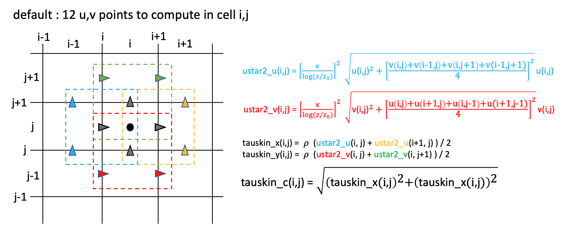
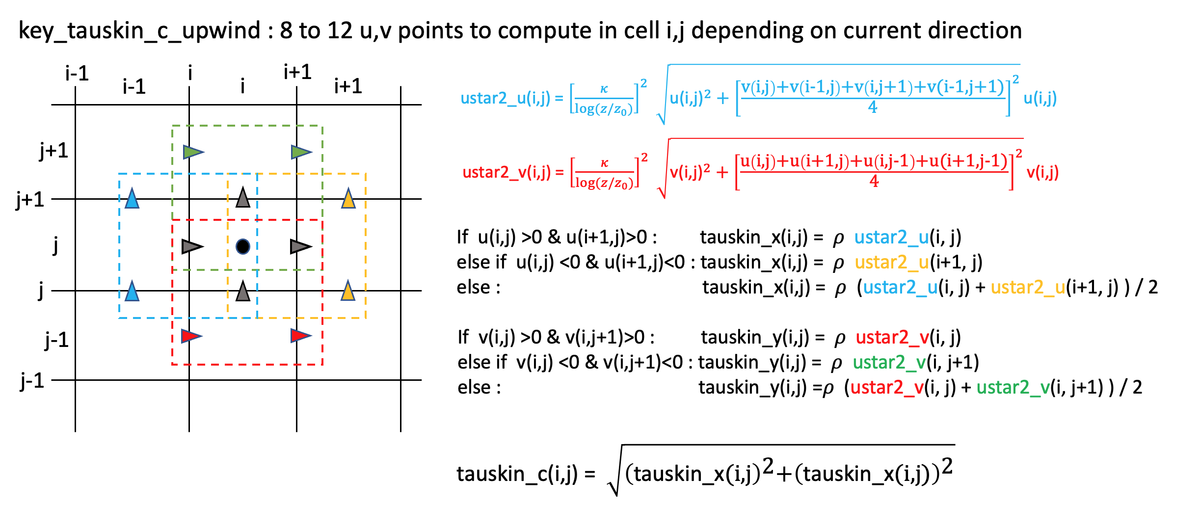
default : compute \(u^*\) components at (u,v) locations first and then at the center of the cell. This option use 12 points of current components (see figure below).
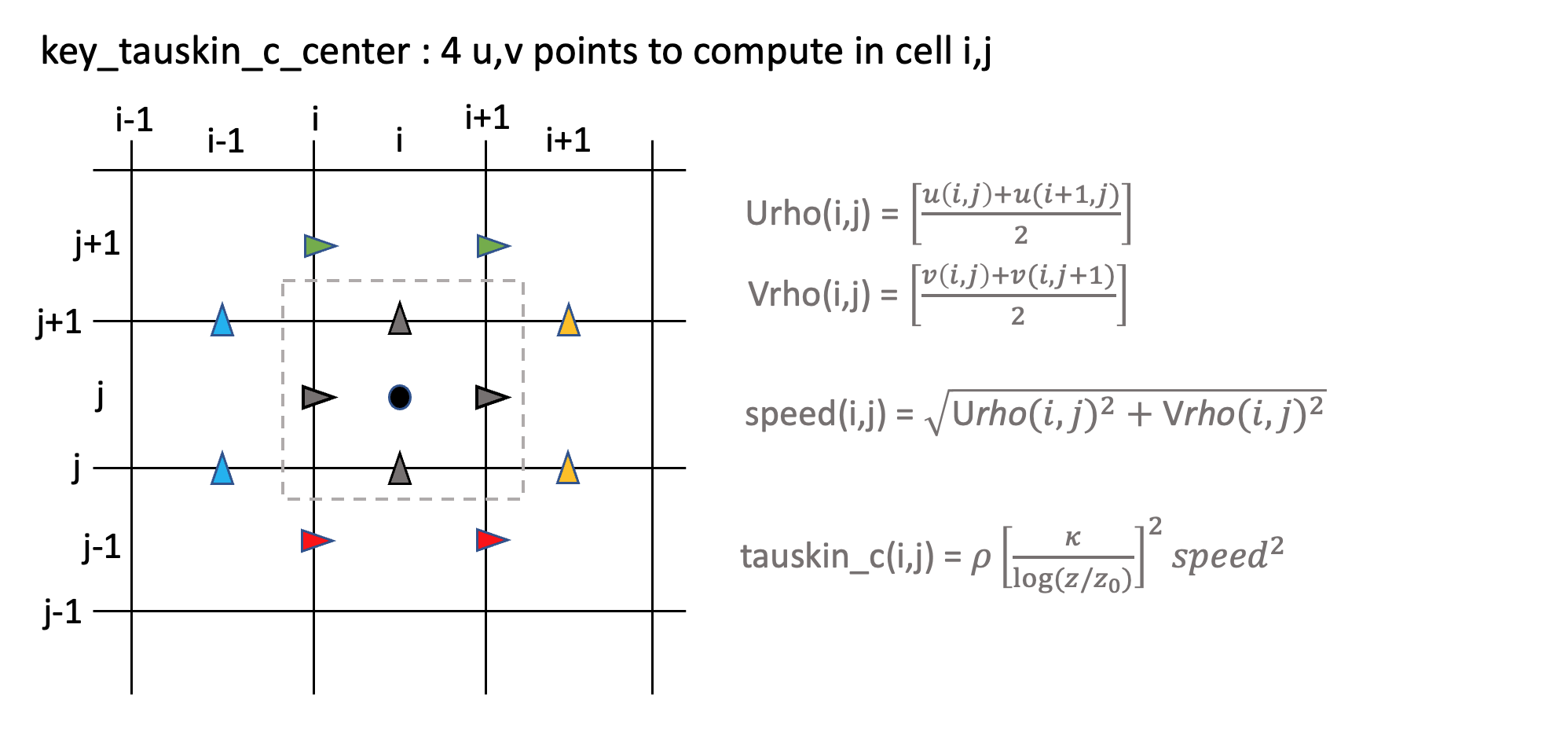
key_tauskin_c_center : compute \(u^*\) directly at (rho) location (center of the cell) using immediate u,v components. This option use 4 points of current components (see figure below).
key_tauskin_c_ubar : compute \(u^*\) using ubar,vbar value instead of bottom layer u,v values.
key_tauskin_c_upwind : depending on current direction, use only component upwind (not combinable with key_tauskin_c_center). This option use 8 to 12 points of current components (see figure below).
BBL : computation is done via BBL module of CROCO using constant roughness (from 160 microns diameter). This option is not recommended with MUSTANG due to constant roughness.
Wave skin friction
Wave skin friction is computed using Soulsby (1997) formula.
\(tauskin\_wave = \frac{1} {2} \cdot \rho_w \cdot f_w \cdot Uwave^2\)
With
\(f_w\) equal to fricwav namelist namsedim_bottomstress value or computed from WAVE_OFFLINE file variables (\(Uwave\) and \(Pwave\)) and roughness if l_fricwave namelist namsedim_bottomstress value is True using \(f_w = 1.39 \cdot (\frac{Uwave \cdot Pwave} {2 \cdot \pi \cdot z0sed}) ^ {-0.52}\)
\(Uwave\) and \(Pwave\) reading from WAVE_OFFLINE file
Combinaison of current and wave stresses
Combinaison of current and wave stresses is done from Soulsby (1997) (Dynamics of marine sands - eq.69 and 70 page 92), \(tauskin\) equal to \(tau\_max\)
\(tau\_mean = tauskin\_current \cdot \left( 1 + 1.2 \cdot \left( \frac{tauskin\_wave} { tauskin\_current + tauskin\_wave} \right)^{3.2} \right)\)
\(tau\_max = \sqrt{ \left( tau\_mean + tauskin\_wave \cdot |cos(phi)| \right)^2+ \left(tauskin\_wave \cdot |sin(phi)| \right)^2 }\)
With \(phi\) angle between current and wave.
Note
abs() is used on cos() and sin() because of alternative direction of tau_w in the vector addition of tau_c and tau_w (see Sousby 1997 (Dynamics of marine sands - figure 16 page 89))
12.2.2.3.6. Settling
The settling process is taken into account during the advection-diffusion scheme in the water column and in the exchange from water to sediment via the deposit fluxes.
Settling velocity modelling strategy
The settling velocity is the main variable of the settling process and is moddelled differently for each substance type :
GRAV : gravels are not transported in suspension, they have no settling velocity because they are not in the water column
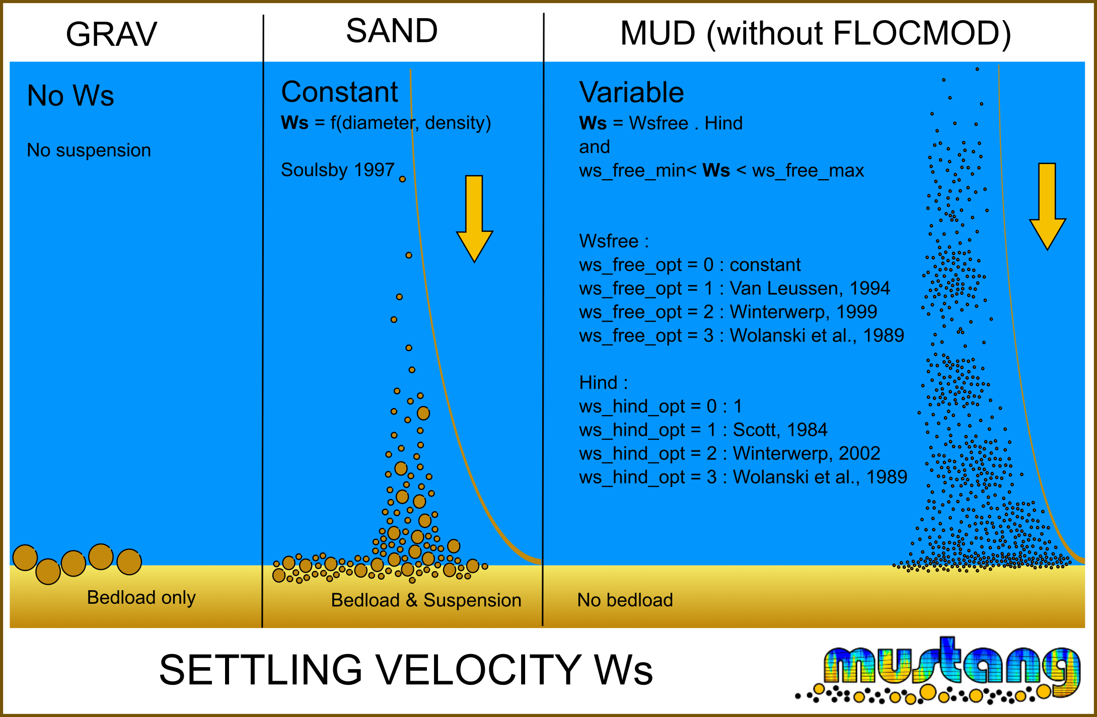
SAND : sands have a constant settling velocity directly compute from Soulsby (1997) using their diameters defined in SUBSTANCE namelist &nmlsands (diam_n).
\(Ws = 10^{-6} \cdot \frac{(107.33 + 1.049 \cdot Dstar^3 )^{0.5} -10.36}{D}\)
With \(Dstar = D \cdot 10^4 \cdot (g\cdot(\frac{\rho_s}{\rho_w}-1))^\frac{1}{3}\) the dimensionless diameter of sediment and D diameter of sediment class, \(\rho_w\) water density and \(\rho_s\) sediment density.
The resulting settling velocity could be high.
MUD and Non Constitutive Particulate subtances : the settling velocity can vary in time and space depending on the parameters chosen by user in SUBSTANCE namelist &nmlmuds: ws_free_opt_n(), ws_free_min_n(), ws_free_max_n(), ws_free_para_n(1:4,num substance), ws_hind_opt_n(), ws_hind_para_n(1:2,num substance) ) or by cpp key for flocculation module (see Flocculation)
If flocculation module is not used, settling velocity is the result of the choice on ws_free_opt_n and ws_hind_opt_n values in SUBSTANCE namelist &nmlmuds and is computed for every cell “i,j” and layer “k” in the water domain.
\(Ws = max( ws\_free\_min\_n\ ;\ min( ws\_free\_max\_n\ ;\ Ws_{free} \cdot Hind))\)
See appropriate chapters for details on free settling velocity and hindered settling parameter.
Sorbed substances : the settling velocity of sorbed substance is the same as the particulate susbtance to which it is associated
Dissolved and fixed substances : no settling velocity
Free settling velocity
\(Ws_{free}\) the free settling velocity is computed from :
if ws_free_opt_n = 0 : constant value, \(Ws_{free} = ws\_free\_min\_n\)
if ws_free_opt_n = 1 : formulation of Van Leussen, 1994, \(Ws_{free} = kC^m \cdot \frac{1 + aG}{1 + b G^2}\)
With :
\(k = ws\_free\_para\_n(1)\) (= 0.0005 in the reference)
\(m = ws\_free\_para\_n(2)\) (= 1.2 in the reference)
\(a = ws\_free\_para\_n(3)\) (= 0.3 in the reference)
\(b = ws\_free\_para\_n(4)\) (= 0.09 in the reference)
\(C\) = Sum of concentration of MUD substances in the layer
\(G = \sqrt{ \frac{turbulence\ dissipation\ rate}{vertical\ viscosity\ coefficient}}\) = turbulence energy
if ws_free_opt_n = 2 : formulation of Winterwerp, 1999, \(Ws_{free} = \frac{1}{18} \cdot \frac{( \rho_s - \rho_w)g}{\rho_w \nu} \cdot Dp^{3-nf} \cdot De^{nf-1}\)
With :
\(De = max( Dp + \frac{ka \cdot C}{kb \cdot \sqrt{G}}\ ;\ \sqrt{\frac{\nu}{G}})\)
\(Dp = ws\_free\_para\_n(1)\) = Primary Particle Diameter, (= 4.10-6 in the reference)
\(ka = ws\_free\_para\_n(2)\) = aggregation factor, (= 14.6 in the reference)
\(kb = ws\_free\_para\_n(3)\) = breakup factor, (= 30000 in the reference)
\(nf = ws\_free\_para\_n(4)\) = fractal dimension, (= 2 in the reference)
\(C\) = Sum of concentration of MUD substances in the layer
\(G = \sqrt{ \frac{turbulence\ dissipation\ rate}{vertical\ viscosity\ coefficient}}\) = turbulence energy
\(\nu = 0.00000102\ m^2/s\) = water kinematic viscosity
\(g\) = gravity
\(\rho_s\) = sediment density
\(\rho_w\) = water density
if ws_free_opt_n = 3 : formulation of Wolanski et al., 1989, \(Ws_{free} = kC^m\)
With :
\(k = ws\_free\_para\_n(1)\) (= 0.01 in the reference)
\(m = ws\_free\_para\_n(2)\) (= 2.1 in the reference)
\(C\) = Sum of concentration of MUD substances in the layer
Hindered settling parameter
\(Hind\) the hindered settling parameter is computed from :
if ws_hind_opt_n = 0 : no hindered effect, \(Hind = 1\)
if ws_hind_opt_n = 1 : formulation of Scott, 1984, \(Hind = (1- \phi)^m\)
With :
\(\phi = min(1\ ;\ \frac{C}{cgel})\)
\(C\) = Sum of concentration of MUD substances in the layer
\(cgel = ws\_hind\_para\_n(1)\) (= 40 in the reference)
\(m = ws\_hind\_para\_n(2)\) (= 4.5 in the reference)
if ws_hind_opt_n = 2 : formulation of Winterwerp, 2002, \(Hind = (1 - \phi_v)^m \cdot \frac{(1 - \phi)}{(1 + 2.5 \phi_v)}\)
With :
\(\phi = \frac{C}{\rho_s}\)
If ws_free_opt_n is not 2 then \(\phi_v = \frac{C}{cgel}\)
If ws_free_opt_n is 2 then \(\phi_v = \phi \cdot (\frac{De}{Dp})^{3-nf}\)
\(De = max( Dp + \frac{ka \cdot C}{kb \cdot \sqrt{G}}\ ;\ \sqrt{\frac{\nu}{G}})\)
\(Dp = ws\_free\_para\_n(1)\) = Primary Particle Diameter, (= 4.10-6 in the reference)
\(nf = ws\_free\_para\_n(4)\) = fractal dimension, (= 2 in the reference)
\(cgel = ws\_hind\_para\_n(1)\) (= 40 in the reference)
\(m = ws\_hind\_para\_n(2)\) (= 1 in the reference)
\(C\) = Sum of concentration of MUD substances in the layer
\(\rho_s\) = sediment density
if ws_hind_opt_n = 3 : formulation of Wolanski et al., 1989, this formulation has to be combined with ws_free_opt_n = 3.
If ws_free_opt_n is not 3 then no hindered effect \(Hind = 1\)
If ws_free_opt_n is 3 then \(Hind = \frac{1}{(C^2+b_w^2)^{m_w}}\)
With :
\(b_w = ws\_hind\_para\_n(1)\) (= 2 in the reference)
\(m_w = ws\_hind\_para\_n(2)\) (= 1.46 in the reference)
\(C\) = Sum of concentration of MUD substances in the layer
Treatment of high settling velocities : SAND variables
For high settling velocities, the major part of the sediment are concentrated in a thin layer near bottom. The thickness of the bottom layer in water could be unadapted to represent correctly the concentration at bottom. This could lead to an underestimation of deposit fluxes and horizontal transport fluxes.
Furthermore, to avoid numerical instabilities, vertical transport is computed using sub time steps. The number of sub time steps depends on the settling velocity of each substance. For high settling velocities, this could be time consuming.
In MUSTANG, these issues are considered for SAND variables only. It is considered that MUD have too low settling velocities and GRAVEL are not transported in suspension.
That is why three features have been developped for SAND variables in MUSTANG to treat these issues :
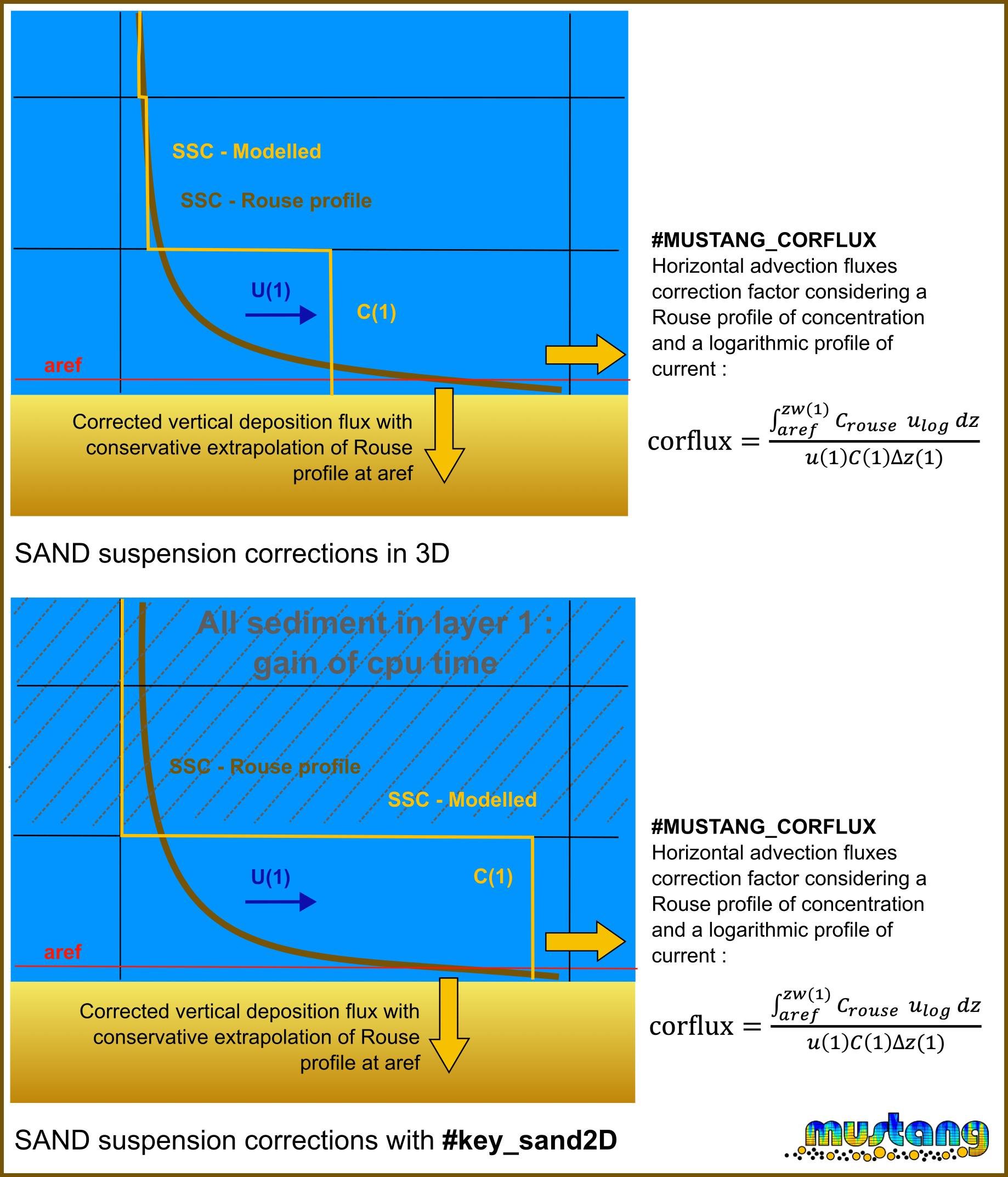
vertical deposit fluxes are corrected considering a Rouse profile in the bottom layer in water. The concentration is extrapolated at a given reference height (parameter aref_sand of MUSTANG namelist) to obtain a correct deposit flow.
horizontal advection fluxes could, as an option, be corrected considering a Rouse profile of concentration and the current logarithmic gradient near bottom. This option is activated by the cpp key MUSTANG_CORFLUX
SAND sediments could, as an option, be considered as 2D variables with the cpp key key_sand2D. When this ccp key key_sand2D is activated, a boolean l_sand2D in SUBSTANCE namelist &nmlsands specify for each SAND substance if it has to be treated as a 2D variable and not 3D. This option makes it possible to treat the fall of SAND-type sediments by considering that the transport in suspension only takes place in the bottom layer (2D sand transport in a single layer). This makes it possible to skip the vertical transport and mixing for this susbtance and save calculation time. As an option (l_outsandrouse in SUBSTANCE namelist &nmlsands), the Rouse profile is reconstructed in the outputs.
The Rouse profile used in those three features involves the ratio Ws/u* to calculate the Rouse number (Z in the formulation below). The formulations used are those proposed by Julie Vareilles (activity report of the post-doctorate Consequences of Climate Change on Ecogeomorphology of Estuaries, March 2013)
Rouse profile:
\(C(z) = C(a) \cdot (\frac{h-z}{z} \cdot \frac{a}{z-a})^{Z}\)
With :
\(a\) : reference height
\(h\) : water height
\(Z\) : Rouse number
For \(\frac{W_s}{u_*}< 0.1\) : \(\beta=1 , Z = \frac{W_s}{\kappa \cdot u_*}\)
For \(0.1 <= \frac{W_s}{u_*}< 0.75\) : \(\beta=1+2(\frac{W_s}{u_*})^2 , Z = \frac{W_s}{\beta \cdot\kappa \cdot u_*}\)
For \(0.75 <= \frac{W_s}{u_*}< 1.34\) : \(Z = 0.35 \frac{W_s}{u_*} + 0.727\)
For \(1.34 <= \frac{W_s}{u_*}\) : \(Z = 1.2\)
12.2.2.3.7. Flocculation with FLOCMOD
Introduction
Suspended particulate matter (SPM) dynamics in estuaries and coastal seas is driven by flocculation processes. These processes modify floc sizes and floc densities, and hence their settling velocity. This parameter is crucial when modelling SPM transport in coastal systems. It can be set as a constant value, or evaluated though an empirical function (such as Van Leussen relationship, see settling velocity chapter) to mimic flocculation dynamics with processes “at equilibrium”.
FLOCMOD is a 0D size-class-based module developed by Ifremer to simulate the explicitly flocculation processes (See Verney et al., 2011). It based on the population equation system originally proposed by Smoluchowski (1917). As a size class-based model, this means that the floc size distribution is represented by a discrete number of sediment classes of increasing sizes. This module simulates the effect of turbulence and SPM concentration and flocculation processes, and uses the fractal approach to represent main floc properties (floc density, floc mass, floc settling velocity).
Future developments are scheduled to include seasonal variability in organic matter content and hence modulate flocculation processes, and floc resistance to breakup for instance.
Module description
FLOCMOD in CROCO
FLOCMOD is available in CROCO using the SEDIMENT (USGS) module or the MUSTANG module. Using MUSTANG, FLOCMOD is activated with the cppkey #key_mustang_flocmod. The MUSTANG specific cppkeys must also be activated.
Floc size classes are defined as mud types in SUBSTANCE namelist parasubstance_MUSTANG.txt. The floc diameter in the namelist correspond to the floc size of the given class. Update the number of sediment classes in param.h (ntrc_sub) accordingly. You may also update obc and input files and sediment initial distribution file if you want to prescribe a specific floc size distribution from rivers or open boundary conditions. Floc sizes are discrete classes, which means that floc created by aggregation or fragmentation is redistributed along the two nearest classes (in floc mass) using a mass-conservative interpolation scheme based on inverse distance.
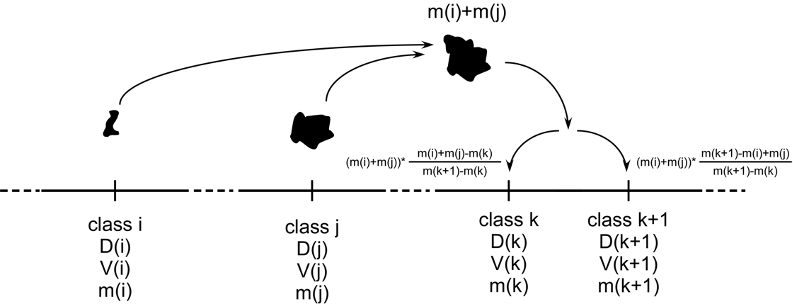
Flocmod redistribution on discrete classes
FLOCMOD parameters are all defined in MUSTANG namelist within the flocmod namelist namflocmod. The different parameters are listed and detailed below when describing flocculation processes.
To save computation time, probability kernels are mainly pre-processed before the computation loop, except the fragmentation by collision kernel. Be careful, if l_COLLFRAG is activated, computation time can be very significantly impacted.
FLOCMOD processes
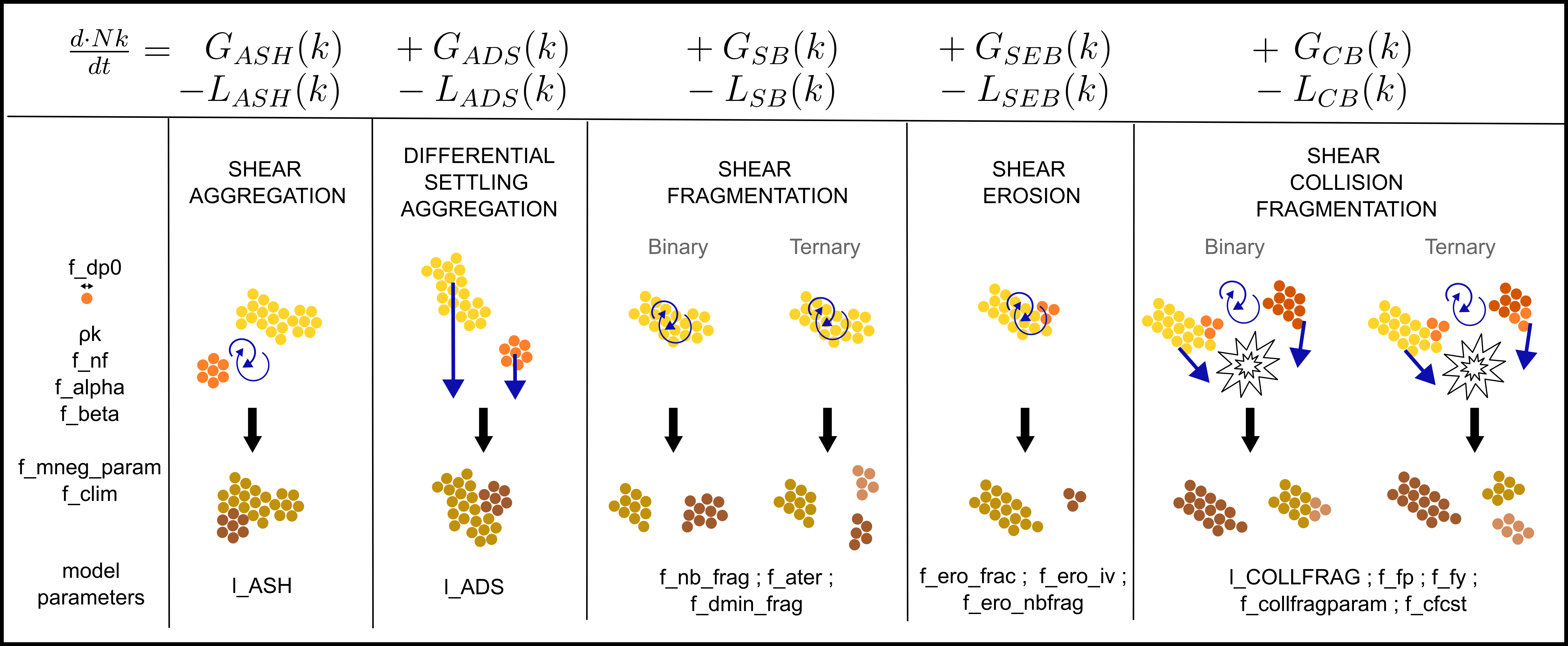
Flocculation processes are actually competition between aggregation and breakup mechanisms, driven by turbulence, SPM concentration, and potentially salinity and organic matter content. The last two control parameter are not yet included in FLOCMOD explicitly. Aggregation is controlled by turbulent shear and differential settling, while fragmentation is exclusively controlled by shear, with different (concurrently usable) options: shear fragmentation, shear erosion, collision-induced fragmentation. All floc interactions are limited to “two-body” interactions. The generic equation given below define all processes involved in FLOCMOD, both in term of gain (G) or loss (L) per class. The main model variable is the number concentration of flocs Nk in a given class k. ASH, ADS and fragmentation by collision can be activated using boolean l_ASH, l_ADS and l_COLLFRAG respectively from the namelist.
Flocmod processes
Floc fractal approach
Flocs observed in nature are characterized by a wide range of size and densities, based on mineral intrinsic features, the organic matter content in SPM, and based on hydrological and hydrodynamics factors. In general, small flocs have high excess densities (O(100-1000 kg/m3)), and large flocs low densities (O(10-100kg/m3)). In FLOCMOD, we use the fractal approach to represent floc characteristics (Kranenburg, 1994) : floc size D, floc mass M, floc excess density \(\Delta \rho\) (\(\rho - \rho_w\)). Flocs are formed from N primary particles with a unique size \(D_p\) (f_dp0 in the namelist) and density \(\rho_p\) (ros from the SUBSTANCE namelist parasubstance_MUSTANG.txt). The floc structure (~compacity) is controlled by the fractal dimension \(n_f\) (f_nf) such as:
\(N = (\frac{D} {D_p})^n_f\)
\(M = \rho_p \cdot \frac{\pi} {6} \cdot {D_p}^3 \cdot N\)
\(\Delta \rho = (\rho_p - \rho_w) \cdot (\frac{D} {D_p})^{3-n_f}\)
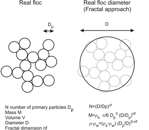
Flocmod fractal approach
Shear rate G
The shear rate G is an hydrodynamic parameter. If GLS_MIXING cppkey is used in CROCO, G can be directly calculated from \(\epsilon\) such as :
\(G = \sqrt{\frac{\epsilon}{\nu}}\)
Otherwise, an \(\epsilon\) vertical profile is calculated from Nezu and Nakagawa and the bottom friction velocity \(u^*\) (from MUSTANG) such as :
\(\epsilon = \frac{{u^*}^3}{\kappa h} \frac{h-z}{z}\)
Where h is the water depth and z the distance from bottom.
Shear aggregation (\(G_{ASH}\) ; \(L_{ASH}\))
These terms correspond to the gain or loss of class k particles when i) two particles in movement (by shear) collide and ii) the collision is efficient, i.e. the newly formed bound between the two particles can withstand the shear induced by the collision. The two-body collision probability function \(A_{SH}(i,j)\) is a function of the shear rate \(G\) and particle diameters \(D_i\) and \(D_j\) (McAnally andMehta,2001,2002)
\(G_{ASH}(k) = \frac{1}{2} \sum_{M_i+M_j=M_k} \alpha_{ij} A_{SH}(i,j) n_i n_j\)
\(L_{ASH}(k) = \sum_{i=1}^{nc} \alpha_{ik} A_{SH}(i,k) n_i n_k\)
\(A_{SH}(i,j) = \frac{G}{6} (D_i + D_j)^3\)
\(\alpha_{ij}\) is the collision efficiency representing particle cohesiveness, i.e. the physico-chemical forces and the sticking properties of organic matter. In the actual version of FLOCMOD, \(\alpha_{ij} = \alpha\) is a constant parameter (between 0 and 1) set in the FLOCMOD namelist.
Differential settling aggregation (\(G_{ADS}\) ; \(L_{ADS}\))
\(A_{DS}\) represents collisions and aggregation that can occur when 2 flocs with different settling velocities can interact during settling. Kernels are similar to \(G_{ASH}\) and \(L_{ASH}\), except that the collision probability \(A_{SH}\) is substituted with \(A_{DS}\) such as :
\(A_{DS}(i,j) = \frac{\pi}{4} (D_i + D_j)^2 \mid W_{s,i} - W_{s,j} \mid\)
Where \(W_{s,i}\) is the floc settling velocity of class i, calculated from Stokes :
\(W_{s,i} = \frac{g}{18 \mu} \Delta\rho_i {D_i}^2\)
Shear fragmentation (\(G_{SB}\) ; \(L_{SB}\))
Shear fragmentation represents the action of shear (turbulent) forces on flocs, leading to breakup.
\(G_{SB}(k) = \sum_{i=k+1}^{nc} FDSB_{ki} B_i n_i\)
\(L_{SB}(k) = B_k n_k\)
\(B_i = \beta_i G^{\beta_2} D_i (\frac{D_i - D_p}{D_p})^{\beta_3}\)
\(\beta_i\) is the fragmentation rate, indirectly related to yield strength and floc resistance to breakup. In the actual version of FLOCMOD, \(\beta_i\) is a constant set in the FLOCMOD namelist. Following Winterwerp (2002), beta_2 = 3/2 and beta_3 = 3 - n_f.
FDSB is the size distribution function of fragmented flocs by shear. Two modes are available: binary or ternary breakup.
Binary distribution : fragmentation of a floc with mass \(m_i\) in two identical flocs of mass \(m_i/2\).
\(FDSB_{ij} = \left\{\begin{array}{ll}2 & \mbox{if } m_j = \frac{m_i}{2} \\0 & \mbox{otherwise}\end{array}\right.\)
Ternary distribution : fragmentation of a floc with mass \(m_i\) in one floc of mass \(m_i/2\) and 2 flocs of mass \(m_i/4\).
\(FDSB_{ij} = \left\{\begin{array}{ll}1 & \mbox{if } m_j = \frac{m_i}{2} \\2 & \mbox{if } m_j = \frac{m_i}{4} \\0 & \mbox{otherwise}\end{array}\right.\)
In FLOCMOD, binary fragmentation is activated if f_nb_frag = 2 and f_ater = 0, and ternary fragmentation if f_nb_frag = 2 and f_ater = 0.5; Shear breakup can be only applied from a given floc size to limit fragmentation for small flocs. This can be set in FLOCMOD by changing f_dmin_frag.
Erosion fragmentation
Shear fragmentation by floc erosion is an additional option to represent floc breakup. In this case, flocs are not broken by 2 or 4 but a small fraction of the floc mass is eroded from the parent floc. This mode transfers a part of the shear fragmentation probability to floc erosion using f_ero_frac. This means that (1-f_ero_frac) contributes to binary/ternary fragmentation and f_ero_frac to fragmentation by erosion.
\(G_{SEB}\) and \(L_{SEB}\) are calculated identically to \(G_{SB}\) and \(L_{SB}\), except that the fragmentation distribution changes according to the floc erosion parameter (FDSEB instead of FDSB) :
\(FDSEB_{ij} = \left\{\begin{array}{ll}1 & \mbox{if } m_j = m_i - f\_ero\_nbfrag \cdot m_i \\2 & \mbox{if } m_j = m_i \\0 & \mbox{otherwise}\end{array}\right.\)
Collision fragmentation
Collision can not only contribute to form bigger flocs, but instead if turbulence is strong, collision can overpass floc strength and then contribute to break particles by mechanical failure. Hence, when activating this option, part of the collision probability (\(A_{SH}(i,j)\)) can induce fragmentation.
\(G_{CB}(k) = \sum_{i=1}^{nc} \sum_{j=i}^{nc} FDCB_{ij} \cdot A_{SH}(i,j) \cdot n_i \cdot n_j\)
\(L_{CB}(k) = \sum_{i=1}^{nc} FDCB_{ik} \cdot A_{SH}(i,k) \cdot n_i \cdot n_k\)
\(FDCB_{ij}\) is the distribution of flocs after collision, and is function of the floc strength \(\tau_{y,i}\) and the collision-induced shear stress between floc i and j : \(\tau_{collij,i}\).
\(\tau_{collij,i} = \frac{8}{\pi} \frac{(G \frac{D_i + D_j}{2})^2}{F_p \cdot {D_i}^2 (D_i + D_j)} \frac{M_i \cdot M_j}{M_i+M_j}\)
\(\tau_{y,i} = F_y \frac{\Delta\rho_i}{\rho_w}^\frac{2}{3-nf}\)
Fp and Fy can be user-defined in the FLOCMOD namelist as f_fp and f_fy respectively.
For two-body interactions (i and j), two types of failures are likely to happen and control the expression of \(FDBC_{ij}\) (McAnally, 1999):
Collision fragmentation #1 : \(\tau_{y,i} > \tau_{collij,i}\) and \(\tau_{collij,i} > \tau_{y,j}\) : the collision-induced shear stress exceeds the shear strength of the weakest aggregate only, consequently during the collision, the j floc breaks into two fragments (\(F_{j,1}\) and \(F_{j,2}\)) such as \(MF_{j,1} = (1-cfcst) \cdot Mj\) and \(MF_{j,2} = cfcst \cdot Mj\). \(F_{j,1}\) is a free fragment while \(F_{j,2}\) is bound with the i floc. cfcst is the inter-penetration depth, fixed as 3/16 based on McAnally (1999). This parameter is found in the namelist as f_cfcst.
Collision fragmentation #2 : \(\tau_{y,i} < \tau_{collij,i}\) and \(\tau_{collij,i} > \tau_{y,j}\) : the shear stress is larger than shear strength of both i and j flocs. Both flocs break into two fragments (\(F_{i,1}\); \(F_{i,2}\)) and (\(F_{j,1}\); \(F_{j,2}\)) such as \([m_F{i,1}; m_F{j,1}]=(1-cfcst) [M_j; M_j]\) and \([M_F{i,2} ;m_F{j,2}]=cfcst [M_j; M_j]\). Two particles are formed from the two parent flocs \(F_{i,1}\) and \(F_{j,1}\). A third flocs is formed from the two fragments (\(F_{i,2}\) and \(F_{j,2}\)) that bound during collision.
The fraction of collision contributing to floc breakup is controlled through the parameter f_collfragparam.
FLOCMOD execution
FLOCMOD can be non-conservative for high shear rates and/or high SPM concentration. To prevent for instabilities, FLOCMOD includes a sub-time step algorithm. After mass exchange due to flocculation, FLOCMOD checks if the new floc size distribution is fully positive or null. If true, execution continues. Otherwise, the time step is divided by two and a new floc size distribution is recalculated. This time-step adaptation is applied as long as floc size distribution contains negative mass. Flocculation is then repeated until reaching a cumulated time step corresponding to the CROCO time step.
It is possible to be slightly permissive and allow a small negative mass concentration (f_mneg_param). In this case, the class characterized by negative mass is set to 0 and the “corresponding added mass” is proportionally removed from the positive classes to be mass conservative. This can help to limit time step adaptation, and hence reduce computation costs.
It is also possible to disconnect FLOCMOD when SPM concentration is very low. In FLOCMOD, this concentration threshold (in g/l) is defined in f_clim and set by default to 0.001 g/l.
12.2.2.3.8. Erosion process
Note
Patience, work in progress, meanwhile see : https://mars3d.ifremer.fr/docs/doc_MUSTANG/doc.MUSTANG.erosion.html
Erosion fluxes
Lateral erosion
key_MUSTANG_lateralerosion
Note
Patience, work in progress
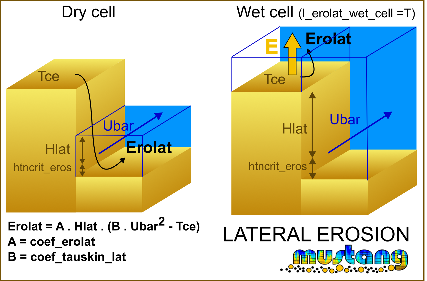
Erosion, layer managment
12.2.2.3.9. Deposit process
Note
Patience, work in progress, meanwhile see : https://mars3d.ifremer.fr/docs/doc_MUSTANG/doc.MUSTANG.deposit.html
Deposit processes are treated implicitly in water transport equations. First, deposition flux trends are evaluated for each variable before advection computations.
Then after advection resolution, effective deposit is computed with new concentrations in water (estimated after transport and settling) and sediment layers are updated (see Deposition layer managment)
Deposit fluxes
TODO : add formulation used for deposit fluxes
Sliding fluxes
A sliding process of the fluid mud is implemented. Only MUD sediments are concerned by this feature. The modelling strategy consists in :
compute the part of mud which slides if the slope is steep
deposit this part towards lower neighboring cells according to the slope
To activate this behavior, the cppkey #key_MUSTANG_slipdeposit must be define and the slopefac value in MUSTANG namelist &namsedim_deposition must be greater than 0.
The part of mud which slides on each cell limit is the product of the slope by the deposit fluxe for each mud class in the cell and by the factor slopefac.
No sediment slides if the slope is not positive.
The sum of sliding sediment over the four cell’s limits could not be greater than the deposit flux computed in the cell.
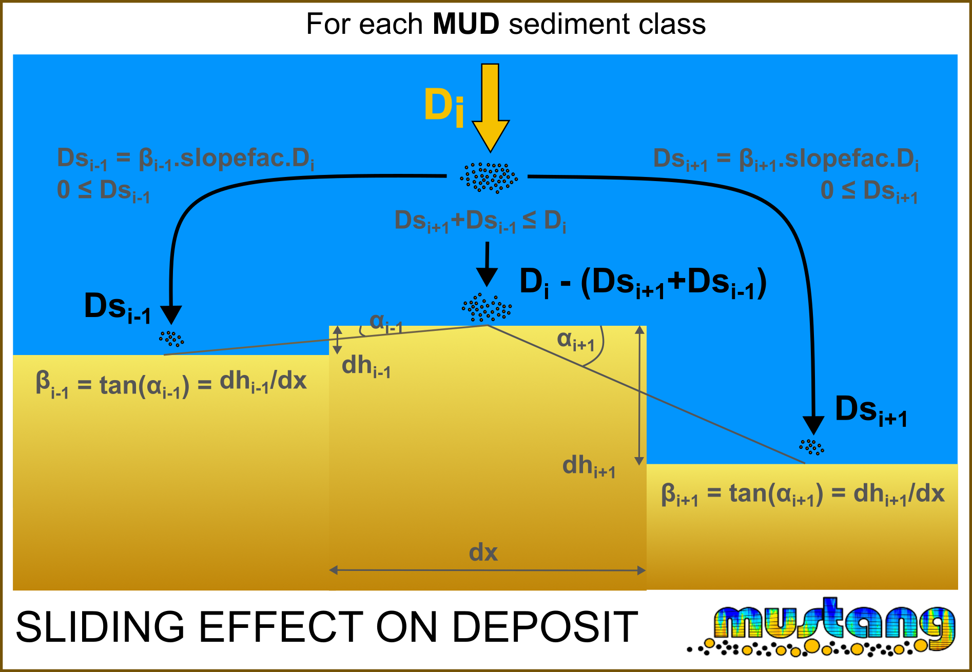
Deposit layer managment
Note
Patience, work in progress
12.2.2.3.10. Consolidation
Cpp keys involved : #key_MUSTANG_add_consol_outputs
Warning
NOT TESTED YET IN CROCO Documentation to come after. Meanwhile : https://mars3d.ifremer.fr/docs/doc_MUSTANG/doc.MUSTANG.consol.html
12.2.2.3.11. Diffusion within sediment and at interface
Cpp keys involved : #key_noTSdiss_insed #key_nofluxwat_IWS
Warning
NOT TESTED YET IN CROCO Documentation to come after. Meanwhile : https://mars3d.ifremer.fr/docs/doc_MUSTANG/doc.MUSTANG.diffu.html
12.2.2.3.12. Bioturbation
Warning
NOT TESTED YET IN CROCO Documentation to come after. Meanwhile : https://mars3d.ifremer.fr/docs/doc_MUSTANG/doc.MUSTANG.bioturb.html
12.2.2.3.13. Morphodynamic
To activate morphodynamic means that the bathymetry used in the hydrodynamic model will evoluate with time. The following figure shows the difference between a non-morphodynamic (ie morphostatic) simulation and a morphodynamic simulation.
The user needs to activate cpp key #MORPHODYN and to set to true the boolean l_morphocoupl (see &namsedim_morpho) to run in morphodynamic mode.
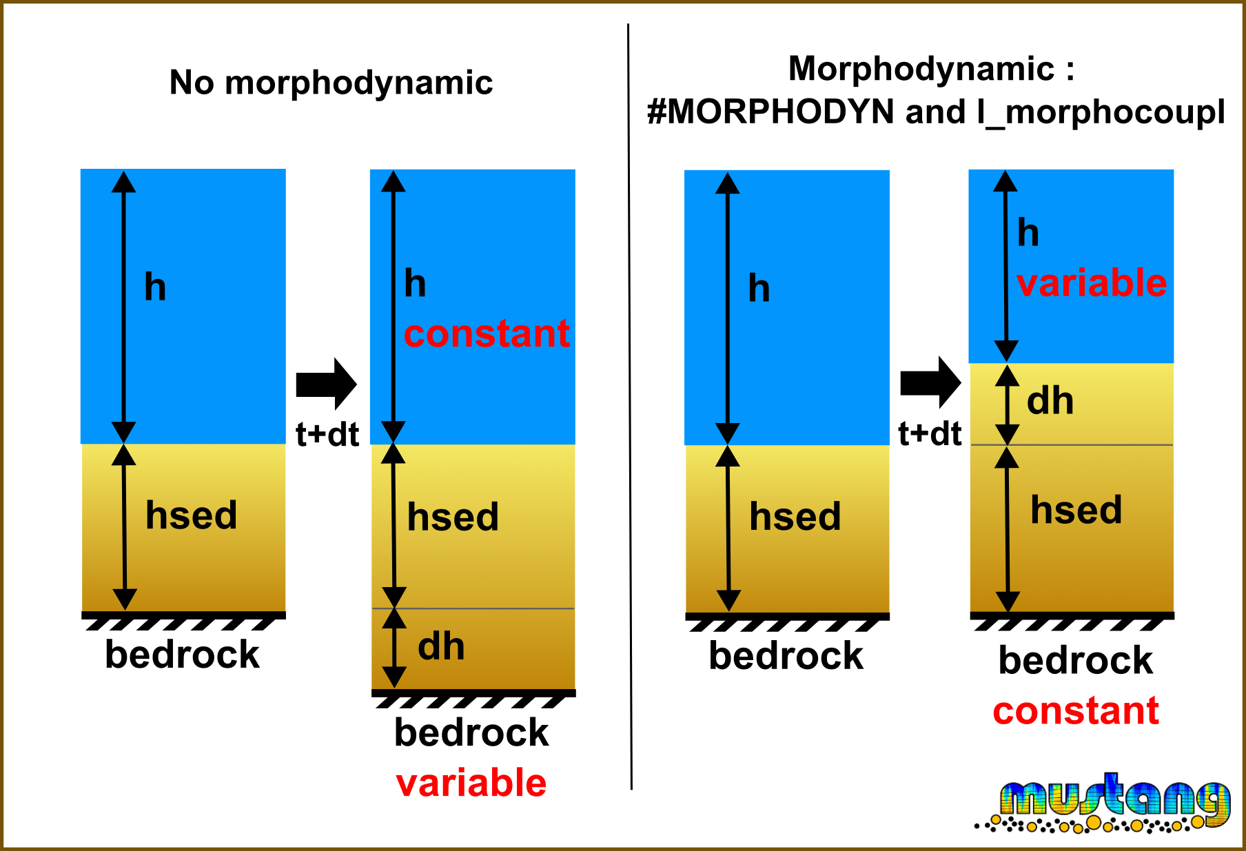
The user can also accelerate morphologic evolution by using MF parameter (see &namsedim_morpho). In this case, two option are available to accelerate the changes :
MF could amplified directly sediment height variation (l_MF_dhsed = T) on water height. In this case, sediment height and the bed layers compositions are not modified. Bedrock location is modified.
MF could amplified erosion/deposition fluxes (l_MF_dhsed = F). In this case, depending on sediment classes in the simulation, the bed layer composition could be different from the case without MF or with (l_MF_dhsed = T) as coarse sediment settled before small one. Sediment height and bed layers compositions are modified but bedrock location is maintained.
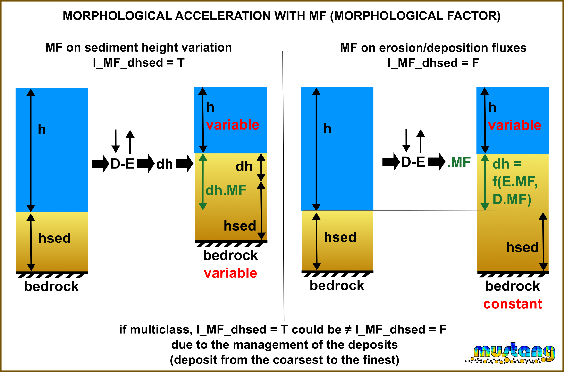
12.2.2.4. FAQ and known issues
Note
Patience, work in progress
V1 or V2 what difference ?
V2 with no sed
River + l_sand2D
Sand in 3D : CPU time
12.2.2.4.1. Coarse sediment in MUSTANG
In MUSTANG V1 (#key_MUSTANG_V2 is not defined), GRAVEL can not go in suspension, they will not move. Another way to deal with GRAVEL in V1 is to declare them as SAND. They will not travel far anyway in suspension, but at least they will impact the sediment dynamics. If their diameter is greater than 2 mm, they will not impact the mean critical bed shear stress (i.e. common critical bed shear stress for all sediment classes in V1).
Nevertheless, MUSTANG V2 is recommended to deal with coarse sediment.
12.2.2.4.2. Not yet implemented features
The feature related to the subroutine bathy_actu_fromfile work for MARS3D but have not been translate for CROCO yet.
The influence of high concentrations of particles on water density have not been coded yet.
Consolidation, bioturbation, flocculation , diffusion within sediment and at interface are code but have not been tested yet.
12.2.2.5. MUSTANG references
Mengual Baptiste, Le Hir Pierre, Cayocca Florence, Garlan Thierry (2017). Modelling Fine Sediment Dynamics: Towards a Common Erosion Law for Fine Sand, Mud and Mixtures . Water , 9(8), 564 (1-24) . Publisher’s official version : 2017_official Open Access version : 2017_openaccess
Grasso Florent, Le Hir Pierre, Bassoullet Philippe (2015). Numerical modelling of mixed-sediment consolidation . Ocean Dynamics , 65(4), 607-616 . Publisher’s official version : 2015_official Open Access version : 2015_openaccess
Le Hir Pierre, Cayocca Florence, Waeles Benoit (2011). Dynamics of sand and mud mixtures: a multiprocess-based modelling strategy. Continental Shelf Research, 31(10), S135-S149. Publisher’s official version : 2011_official Open Access version : 2011_openaccess