4.3. Advection Schemes

4.3.1. Lateral Momentum Advection

Related CPP options:

UV_HADV_UP3	Activate 3rd-order upstream biased advection scheme
UV_HADV_UP5	Activate 5th-order upstream biased advection scheme
UV_HADV_C2	Activate 2nd-order centred advection scheme (should be used with explicit momentum mixing)
UV_HADV_C4	Activate 4th-order centred advection scheme (should be used with explicit momentum mixing)
UV_HADV_C6	Activate 6th-order centred advection scheme (should be used with explicit momentum mixing)
UV_HADV_WENO5	Activate WENO 5th-order advection scheme
UV_HADV_TVD	Activate Total Variation Diminushing scheme

Preselected options:

# define UV_HADV_UP3
# undef  UV_HADV_UP5
# undef  UV_HADV_C2
# undef  UV_HADV_C4
# undef  UV_HADV_C6
# undef  UV_HADV_WENO5
# undef  UV_HADV_TVD

These options are set in set_global_definitions.h as the default UV_HADV_UP3 is the only one recommended for standard users.

4.3.2. Lateral Tracer advection

Related CPP options:

TS_HADV_UP3	3rd-order upstream biased advection scheme
TS_HADV_RSUP3	Split and rotated 3rd-order upstream biased advection scheme
TS_HADV_UP5	5th-order upstream biased advection scheme
TS_HADV_RSUP5	Split and rotated 5th-order upstream biased advection scheme with reduced dispersion/diffustion
TS_HADV_C4	4th-order centred advection scheme
TS_HADV_C6	Activate 6th-order centred advection scheme
TS_HADV_WENO5	5th-order WENOZ quasi-monotonic advection scheme for all tracers
BIO_HADV_WENO5	5th-order WENOZ quasi-monotone advection scheme for passive tracers (including biology and sediment tracers)

Preselected options:

# undef  TS_HADV_UP3
# define TS_HADV_RSUP3
# undef  TS_HADV_UP5
# undef  TS_HADV_RSUP5
# undef  TS_HADV_C4
# undef  TS_HADV_C6
# undef  TS_HADV_WENO5
# if defined PASSIVE_TRACER || defined BIOLOGY || defined SEDIMENT
#  define BIO_HADV_WENO5
# endif

TS_HADV_RSUP3 is recommended for realistic applications with variable bottom topography as it strongly reduces diapycnal mixing. It splits the UP3 scheme into 4th-order centered advection and rotated bilaplacian diffusion with grid-dependent diffusivity. It calls for CPP options in set_global_definitions.h for the explicit treatment of bilaplacian diffusion (see below). TS_HADV_RSUP3 is expensive in terms of computational cost and requires more than 30 sigma levels to perform properly. Therefore, for small domains dominated by open boundary fluxes, TS_HADV_UP5 may present a cheaper alternative and good compromise. TS_HADV_RSUP5 is still experimental but allows a decrease in numerical diffusivity compared to TS_HADV_RSUP3 by using 6th order rather than 4th-order centered advection (it resembles in spirit a split-rotated UP5 scheme but the use of bilaplacian rather than trilaplacian diffusion keeps it 3rd order). TS_HADV_C4 has no implicit diffusion and is thus accompanied by rotated Smagorinsky diffusion defined in set_global_definitions.h; it is not recommended for usual applications. For RSUP family, by default the diffusive part is oriented along geopotential.

4.3.3. Vertical Momentum advection

Related CPP options:

UV_VADV_SPLINES	4th-order compact advection scheme
UV_VADV_C2	2nd-order centered advection scheme
UV_VADV_WENO5	5th-order WENOZ quasi-monotone advection scheme
UV_VADV_TVD	Total Variation Diminushing (TVD) scheme

Preselected options:

#ifdef UV_VADV_SPLINES
#elif defined UV_VADV_WENO5
#elif defined UV_VADV_C2
#elif defined UV_VADV_TVD
#else
# define UV_VADV_SPLINES
# undef  UV_VADV_WENO5
# undef  UV_VADV_C2
# undef  UV_VADV_TVD
#endif

4.3.4. Vertical Tracer advection

Related CPP options:

TS_VADV_SPLINES	4th-order compact advection scheme
TS_VADV_AKIMA	4th-order centered advection scheme with harmonic averaging
TS_VADV_C2	2nd-order centered advection scheme
TS_VADV_WENO5	5th-order WENOZ quasi-monotone advection scheme

Preselected options:

#ifdef TS_VADV_SPLINES
#elif defined TS_VADV_AKIMA
#elif defined TS_VADV_WENO5
#elif defined TS_VADV_C2
#else
# undef  TS_VADV_SPLINES
# define TS_VADV_AKIMA
# undef  TS_VADV_WENO5
# undef  TS_VADV_C2
#endif

4.3.5. Adaptively implicit vertical advection

Related CPP options:

VADV_ADAPT_IMP	Activate adapative, Courant number dependent implicit advection scheme
VADV_ADAPT_PRED	Adaptive treatment at both predictor and corrector steps

Preselected options:

#ifdef VADV_ADAPT_IMP
# undef  VADV_ADAPT_PRED
# define UV_VADV_SPLINES
# undef  UV_VADV_C2
# undef  UV_VADV_WENO5
# undef  UV_VADV_TVD
#endif
#ifdef VADV_ADAPT_IMP
# define  TS_VADV_SPLINES
# undef   TS_VADV_AKIMA
# undef   TS_VADV_WENO5
# undef   TS_VADV_C2
#endif

4.3.6. Numerical details on advection schemes

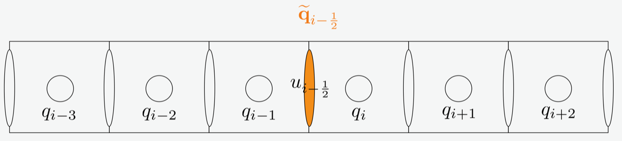
Fig: variable location on an Arakawa C-grid. Tracer values are cell centered while velocities are defined on interfaces.

\[\left. \partial_x( u q ) \right|_{x=x_i} = \frac{1}{\varDelta x_i} \left\{ u_{i+\frac{1}{2}} \widetilde{q}_{i+\frac{1}{2}} - u_{i-\frac{1}{2}} \widetilde{q}_{i-\frac{1}{2}} \right\}\]

4.3.6.1. Linear advection schemes

\begin{eqnarray} \widetilde{q}_{i-\frac{1}{2}}^{\rm C2} &=& \frac{q_i + q_{i-1}}{2} \\ \widetilde{q}_{i-\frac{1}{2}}^{\rm C4} &=& \left(\frac{7}{6}\right) \widetilde{q}_{i-\frac{1}{2}}^{\rm C2} - \left(\frac{1}{12}\right) \left(q_{i+1}+q_{i-2}\right) \\ \widetilde{q}_{i-\frac{1}{2}}^{\rm UP3} &=& \widetilde{q}_{i-\frac{1}{2}}^{\rm C4} + {\rm sign}\left( \frac{1}{12} , u_{i-\frac{1}{2}} \right) \left(q_{i+1} - 3 q_i + 3 q_{i-1} - q_{i-2}\right) \\ \widetilde{q}_{i-\frac{1}{2}}^{\rm C6} &=& \left(\frac{8}{5}\right) \widetilde{q}_{i-\frac{1}{2}}^{\rm C4} - \left(\frac{19}{60}\right) \widetilde{q}_{i-\frac{1}{2}}^{\rm C2} + \left(\frac{1}{60}\right) \left(q_{i+2}+q_{i-3}\right) \\ \widetilde{q}_{i-\frac{1}{2}}^{\rm UP5} &=& \widetilde{q}_{i-\frac{1}{2}}^{\rm C6} - {\rm sign}\left( \frac{1}{60} , u_{i-\frac{1}{2}}\right) \left( q_{i+2} - 5 q_{i+1} + 10 q_i - 10 q_{i-1} + 5 q_{i-2} - q_{i-3} \right) \end{eqnarray}

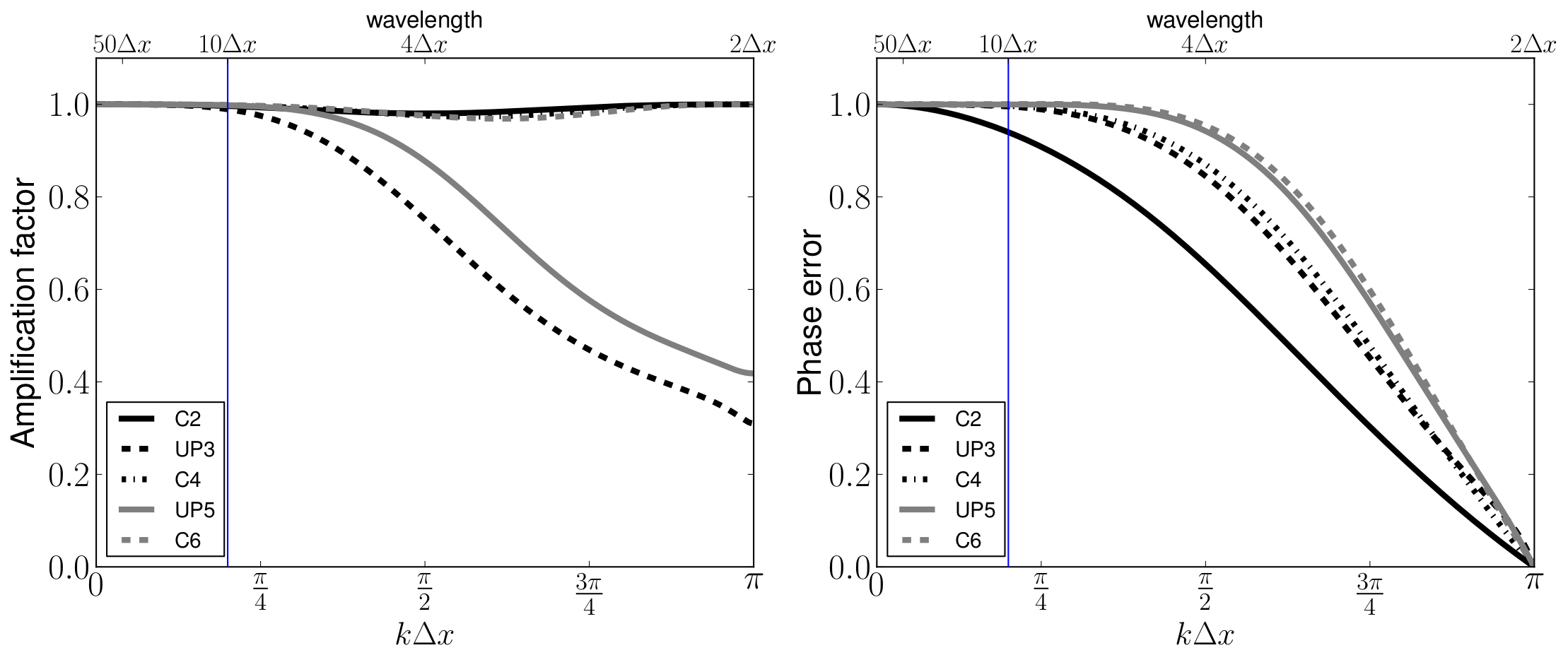
Fig: amplification errors (left) and phase errors (right) for linear advection of order 2 to 6.

4.3.6.2. Split upwind schemes

Because odd-ordered advection schemes can be formulated as the sum of the next higher-order (centered) advection scheme with a dissipation term it is possible to split the purely centered and dissipative parts of UP3 and UP5 schemes. In this case the centered part is treated within the predictor-corrector framework while the flow-dependent dissipative part is treated with a one-step Euler scheme. Such splitting has two advantages:

1. It allows better stability for SUP3 and SUP5 schemes comapared to UP3 and UP5 schemes.

2. Isolating the dissipative part allows to rotate it in the neutral direction to reduce spurious diapycnal mixing (RSUP3 scheme).

4.3.6.3. Splines reconstruction and Akima 4th-order schemes

Similar to a 4th-order compact scheme, the interfacial values for the splines reconstruction scheme are obtained as a solution of a tridiagonal problem

\[{\rm Hz}_{k+1} \widetilde{q}_{k-\frac{1}{2}} + 2 ({\rm Hz}_k + {\rm Hz}_{k+1}) \widetilde{q}_{k+\frac{1}{2}} + {\rm Hz}_k \widetilde{q}_{k+\frac{3}{2}} = 3 ( {\rm Hz}_k \overline{q}_{k+1} + {\rm Hz}_{k+1} \overline{q}_{k} )\]

where \(\overline{q}_{k}\) values should be understood in a finite-volume sense (i.e. as an average over a control volume).

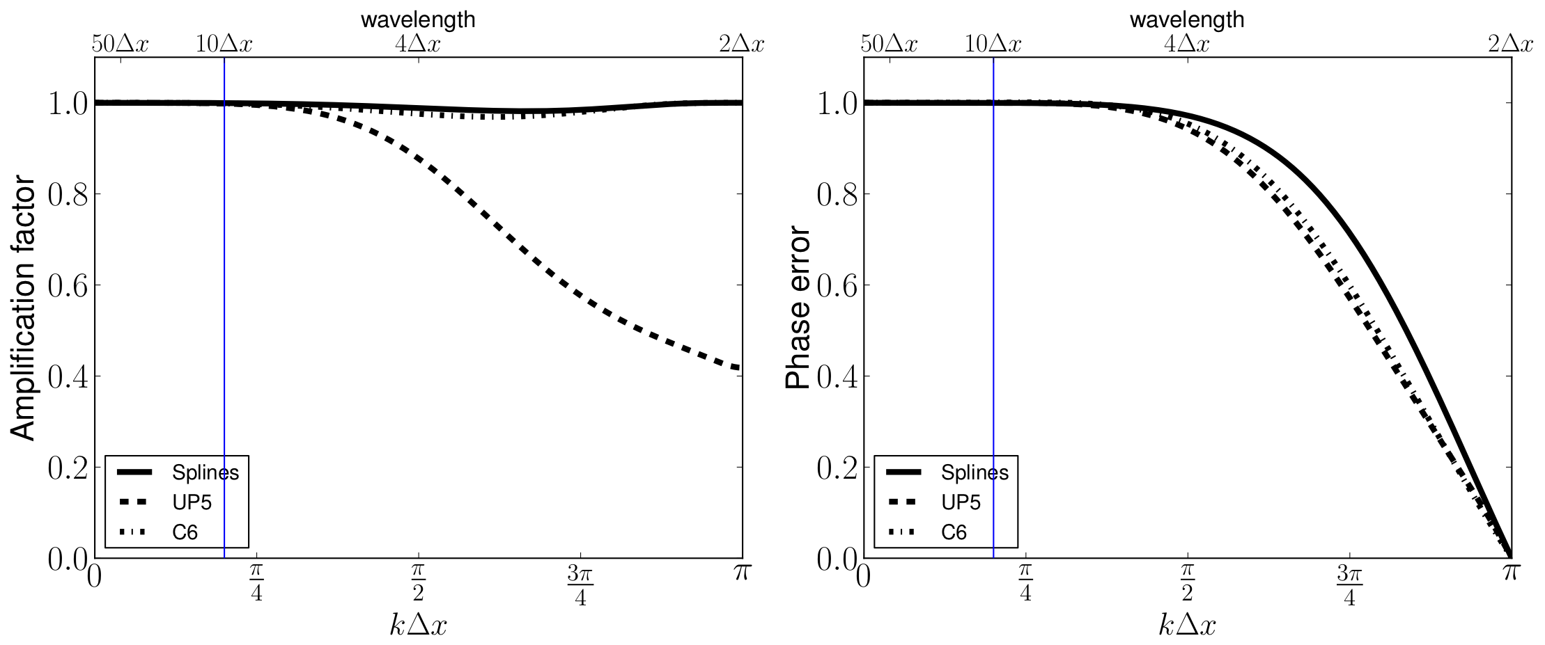
Fig: amplification errors (left) and phase errors (right) for linear advection of order 5 and 6 and for Splines reconstruction.

The AKIMA scheme corresponds to a 4th-order accurate scheme where an harmonic averaging of the slopes is used instead of the algebraic average used for a standard C4 scheme

\[\begin{split}\widetilde{q}_{k+\frac{1}{2}} = \frac{q_{k+1}+q_k}{2} - \frac{\overline{\delta q}_{k+1} - \overline{\delta q}_{k}}{6} \qquad \overline{\delta q}_{k} = \left\{ \begin{array}{cc} \displaystyle 2 \frac{\delta q_{k+\frac{1}{2}} \delta q_{k-\frac{1}{2}}}{\delta q_{k+\frac{1}{2}}+\delta q_{k-\frac{1}{2}}}, & \mbox{if}\;\delta q_{k+\frac{1}{2}} \delta q_{k-\frac{1}{2}} > 0 \\ 0, & \mbox{otherwise}\end{array} \right.\end{split}\]

4.3.6.4. Adaptively implicit vertical advection

Idea: the vertical velocity \(\Omega\) is split between an explicit and implicit contribution depending on the local Courant number

\[\begin{split}\Omega = \mathbf{\Omega^{(e)}} + \mathbf{\Omega^{(i)}}, \qquad \mathbf{\Omega^{(e)}} = \frac{\Omega}{f(\alpha_{\rm adv}^z,\alpha_{\max})}, \quad f(\alpha_{\rm adv}^z,\alpha_{\max}) = \left\{ \begin{array}{ll} 1, & \alpha_{\rm adv}^z \le \alpha_{\max} \\ \alpha / \alpha_{\max}, & \alpha_{\rm adv}^z > \alpha_{\max}\end{array} \right.\end{split}\]

• \(\Omega^{(e)}\) is integrated with an explicit scheme with CFL \(\alpha_{\max}\).

• \(\Omega^{(i)}\) is integrated with an implicit upwind Euler scheme.

• \(f(\alpha_{\rm adv}^z,\alpha_{\max})\) is a function responsible for the splitting of \(\Omega\) between an explicit and an implicit part.

This approach has the advantage to render vertical advection unconditionally stable and to maintain good accuracy in locations with small Courant numbers. The current implementation is based on the SPLINES scheme for the explicit part.

4.3.6.5. Total variation bounded scheme (WENO5)

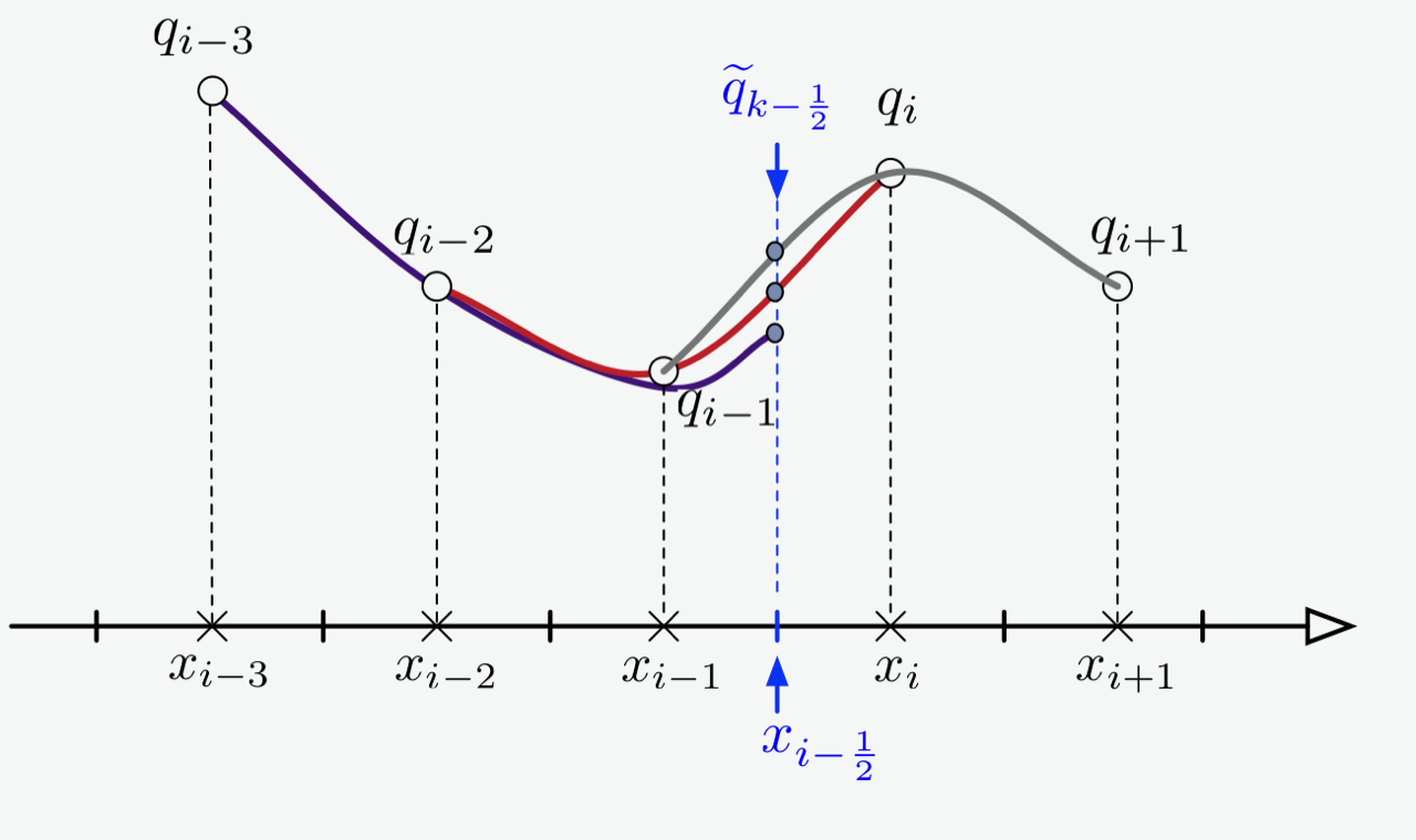
Fig: different stencils used to evaluate the interfacial value \(\widetilde{q}_{k+\frac{1}{2}}\) with WENO5 scheme

Nonlinear weighting between 3 evaluations of interfacial values based on 3 different stencils

\[\widetilde{q}_{k-\frac{1}{2}} = w_0 \widetilde{q}_{k-\frac{1}{2}}^{(0)} + w_1 \widetilde{q}_{k-\frac{1}{2}}^{(1)} + w_2 \widetilde{q}_{k-\frac{1}{2}}^{(2)}\]

where the weights are subject to the following constraints:

1. Convexity \(\sum_{j=0}^2 w_j = 1\).

2. ENO property (Essentially non oscillatory).

3. 5th-order if \(q(x)\) is smooth.

The resulting scheme is not monotonicity-preserving but instead it is Total Variation Bounded (TVB).

4.3.6.6. Total variation diminishing scheme

4.3.6.7. Upwinding of nonlinear terms

In CROCO the nonlinear advection terms are formulated as in Lilly (1965) :

\begin{eqnarray} \partial_t ( {\rm Hz} u ) &+& \partial_x\left( ( {\rm Hz}\; u) u \right) + \partial_y\left( ( {\rm Hz} \; v)\; u \right) + \; ... \\ \partial_t ( {\rm Hz} v ) &+& \partial_x\left( ( {\rm Hz}\; u) v \right) + \partial_y\left( ( {\rm Hz} \; v)\; v \right) + \; ... \end{eqnarray}

which are discretised with third order accuracy as

\begin{eqnarray} \left( \widetilde{( {\rm Hz}\; u) u} \right)_{i,j} &=& ( \widetilde{{\rm Hz}\; u})_{i,j}^{\rm C4} \; \widetilde{u}_{i,j}^{\rm UP3} \\ \left( \widetilde{( {\rm Hz}\; v) u} \right)_{i+\frac{1}{2},j+\frac{1}{2}} &=& ( \widetilde{{\rm Hz}\; v})_{i+\frac{1}{2},j+\frac{1}{2}}^{\rm C4} \; \widetilde{u}_{i+\frac{1}{2},j+\frac{1}{2}}^{\rm UP3} \end{eqnarray}

where the direction for upwinding is selected considering

\[u^{\rm upw}_{i,j} = u_{i+\frac{1}{2},j}+u_{i-\frac{1}{2},j}, \qquad v^{\rm upw}_{i+\frac{1}{2},j+\frac{1}{2}} = ({\rm Hz}\; v)_{i,j+\frac{1}{2}} + ({\rm Hz}\; v)_{i+1,j+\frac{1}{2}}\]