16. Visualization (Python)¶

Croco_visu is a tool written in python to visualize history files genarated by the Croco model.

16.1. Setup your Miniconda environment¶

Download and install miniconda: download Miniconda from the Conda website. See the documentation for installation.
Put the path in your shell environment file (ex:.cshrc, .bashrc)
```
source path_to_your_miniconda/etc/profile.d/conda.csh
```

Create your conda croco_pyvisu environment

conda update conda
conda create -n croco_pyvisu -c conda-forge python=3.7 wxpython xarray matplotlib netcdf4 scipy ffmpeg
conda create --name toto --clone

16.2. Croco_visu directory¶

The croco_pyvisu directory is provided in the CROCO_TOOLS.

16.3. Launch visualization¶

To start croco_visu:

conda activate croco_pyvisu
croco_gui_xarray.py

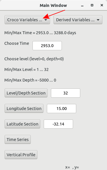
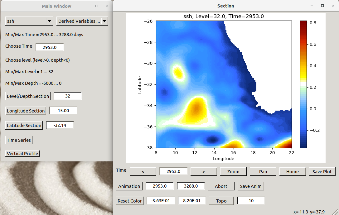
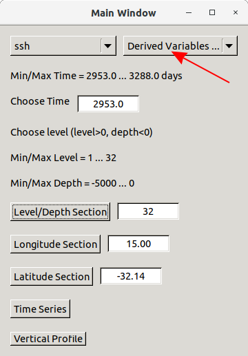
The main window is opened.

First, you have to choose a variable through the Croco Variables… menu, which list all the 2D/3D variables of the history file.

Min/max Time of the file are filled out

You can type a time in the Choose Time input box. The nearest time of the history file will be retrieved.

Warning

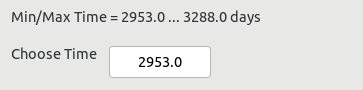
Each time you type something in an input text box, you must validate the input with the Enter key.

Min/max level and min/max depth of the file are indicated

You can type a level or depth in the input level/depth box (>0 means level, <=0 means depth), by default, the value is the highest level

You can type a longitude/latitude in the input longitude/latitude box (default is the mean longitude/latitude)

Now you can click on the Level/Depth Section button and a new window appears.

In this new window, you can only plot the current variable at the current level/depth. If you want another variable, or another level/depth, you have to choose first another variable or another level/depth and click again on the Level/Depth Section button. Then you will have another new window.

This new window offers several buttons and information:

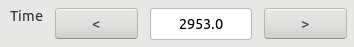
to change the current time, you can type a new time in the text box or use the arrows

to zoom, translate and save the plot

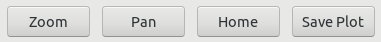To zoom, you have to first click the Zoom button and after select the region to zoom.

To translate the plot, you have to first click the Pan button and then move the plot with the left mouse button.

The Home button is to go back to the default view.

The Save Plot button will open a new window for you to save the current plot.

to create animations

You have first to choose the start time and the end time in the two input text boxes. Then you can click on the Animation button to start the animation. You can abort the animation with the Abort button and if you select the Save Anim button, your animation is saved in a sub-directory Figures_.

change the colorbar

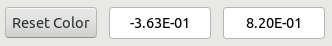You can choose new limits for the colorbar (return to validate the input) or you can go back to the default colorbar with the Reset Color button.

show contours of the topography

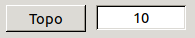You can show the contours of the topography by clicking on the Topo button (on/off) and you can change the number of contours shown in the text input box (return to validate the input, default is 10).

see the coordinates of the current point

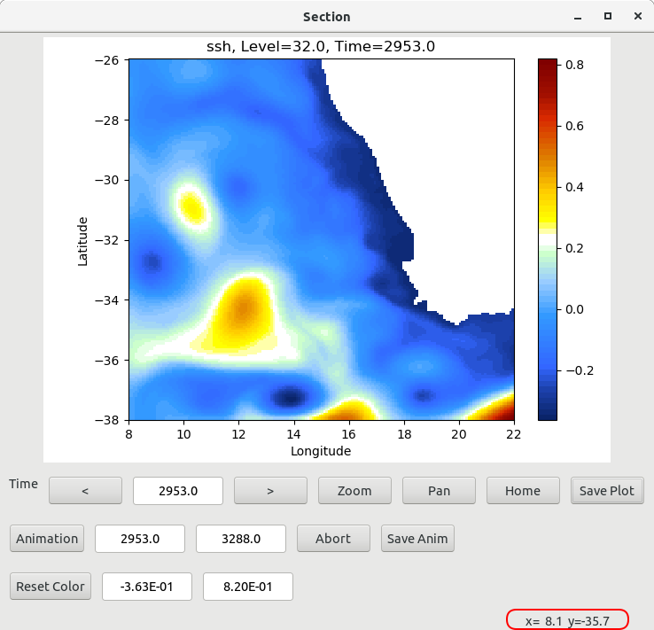At the right bottom corner of the window, you have the coordinates of the cursor.

On the main window, the two others buttons Longitude Section and Latitude Section will open the same kind of window than the Level/Depth Section but at a given longitude or latitude.

Of course, to have a longitude/latitude section, you must choose a 3D variable.

You have to choose first the longitude/latitude before clicking the buttons. The longitude/latitude can be typed in the text input boxes near the buttons, or you can click on a plot to select a new point. If you click on the plot of a

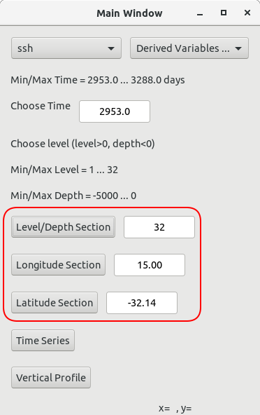
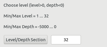
Level/Depth Section, you select new longitude and latitude.
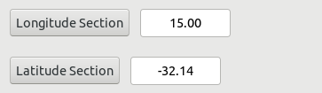
Longitude Section, you select new depth and latitude.
Latitude Section, you select new depth and longitude.

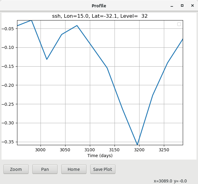
The two last buttons of the main window Time Series and Vertical Profile create new windows to plot curves.

Both Time Series and Vertical Profile have the same possibilities.

Zoom a part of the curve: you must first select the Zoom button and then select the region to zoom.
Pan the curve: you must first select the Pan button and then translate the curve.
Home to go back to the default view
Save Plot : when you click on the Save Plot button, a popup window is opened for you to choose the name of the file.

The time series is plotted at the current level/depth, longitude and latitude. The vertical profile is plotted at the current longitude/latitude.

You also have the coordinates of the cursor at the right bottom of the window.

16.4. How to customize for your own history files¶

The only file you have to change is the file croco_wrapper.py. You have two files as examples in the repository:

croco_wrapper.py.benguela for the Benguela test case, where history files are created through the classic method.

croco_wrapper.py.moz where the history files are created through XIOS.

Choose the right one to start

cp croco_wrapper.py.benguela croco_wrapper.py

Change path and keymap_files to load the right files:

path = "./"
keymap_files = {
    'coordinate_file': path + "croco_his_Y2008.nc",
    'metric_file': path + "croco_his_Y2008.nc",
    'mask_file': path + "croco_his_Y2008.nc",
    'variable_file': path + "croco_his_Y2008.nc"
}

coordinate_file : containing lon_r, lat_r, time
metric_file : containing pm, pn, theta_s, theta_b, Vtransform, hc, h, f
mask_file : containing mask_rho
variable_file : containing ssh, u, v, w, temp, salt, rho

Change the keymap_* dictionnaries to suit your files, you must only change the keys, that is the values on the left before the “:”:

keymap_dimensions = {
    'xi_rho': 'x_r',
    'eta_rho': 'y_r',
    'xi_u': 'x_u',
    'y_u': 'y_r',
    'x_v': 'x_r',
    'eta_v': 'y_v',
    'x_w': 'x_r',
    'y_w': 'y_r',
    's_rho': 'z_r',
    's_w': 'z_w',
    'time': 't'
}


keymap_coordinates = {
    'lon_rho': 'lon_r',
    'lat_rho': 'lat_r',
    'lon_u': 'lon_u',
    'lat_u': 'lat_u',
    'lon_v': 'lon_v',
    'lat_v': 'lat_v',
    'scrum_time': 'time'
}


keymap_variables = {
    'zeta': 'ssh',
    'u': 'u',
    'v': 'v',
    'w': 'w',
    'temp': 'temp',
    'salt': 'salt',
    'rho': 'rho'
}

keymap_metrics = {
    'pm': 'dx_r',
    'pn': 'dy_r',
    'theta_s': 'theta_s',
    'theta_b': 'theta_b',
    'Vtransform': 'scoord',
    'hc': 'hc',
    'h': 'h',
    'f': 'f'
}

keymap_masks = {
    'mask_rho': 'mask_r'
}

16.5. How to add new variables¶

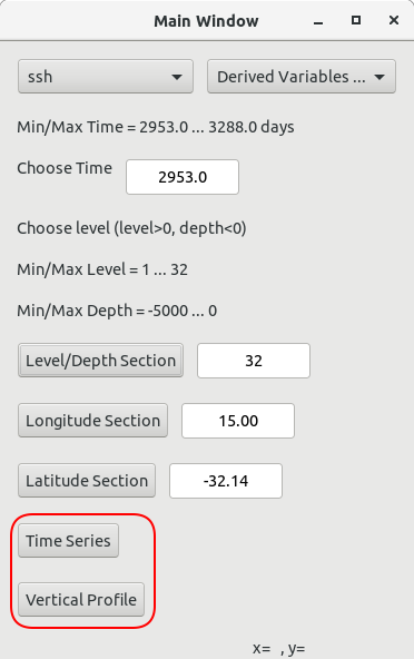
In the main window, you have another menu called Derived Variables…, which contains calculated variables, derived from the base fields found in the history file.

Right now, available variables are

pv_ijk

Ertel potential vorticity is given by \(\frac{curl(u) + f}{rho}\)
zeta_k

zetak is given by \(\frac{\partial{v}/\partial{x} - \partial{u}/\partial{y}}{f}\)
dtdz

dtdz in given by \(\frac{\partial{T}}{\partial{z}}\)
log(Ri)

Ri is given by \(\frac{N²}{(\partial{u}/\partial{z})² - (\partial{v}/\partial{z})²}\) with \(N=\sqrt{\frac{-g}{rho0} * \frac{\partial{rho}}{\partial{z}}}\)

You can add new variables by:

in the file CrocoXarray.py, add a line in the method list_of_derived:

def list_of_derived(self):
    ''' List of calculated variables implemented '''
    keys = []
    keys.append('pv_ijk')
    keys.append('zeta_k')
    keys.append('dtdz')
    keys.append('log(Ri)')
    return keys

in the file derived_variables.py, add two functions get_newvar and calc_newvar to calculate the new variable
in the file croco_gui_xarray.py, add the calls to the new function get_newvar in updateVariableZ, onTimeSeriesBtn and onVerticalProfileBtn