13. Nesting Tutorial¶

Nesting is performed in the model through the AGRIF library.

To create a nested configuration:

First build the parent domain configuration as in previous section
Then in matlab, you need to use the nestgui utility
```
nestgui
```
The nestgui will appear :

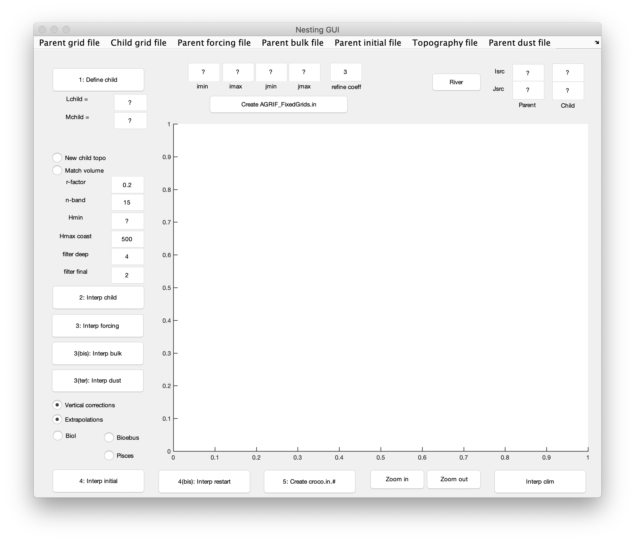
Entrance window of nestgui¶
First choose the grid file of your parent domain: CROCO_FILES/croco_grd.nc.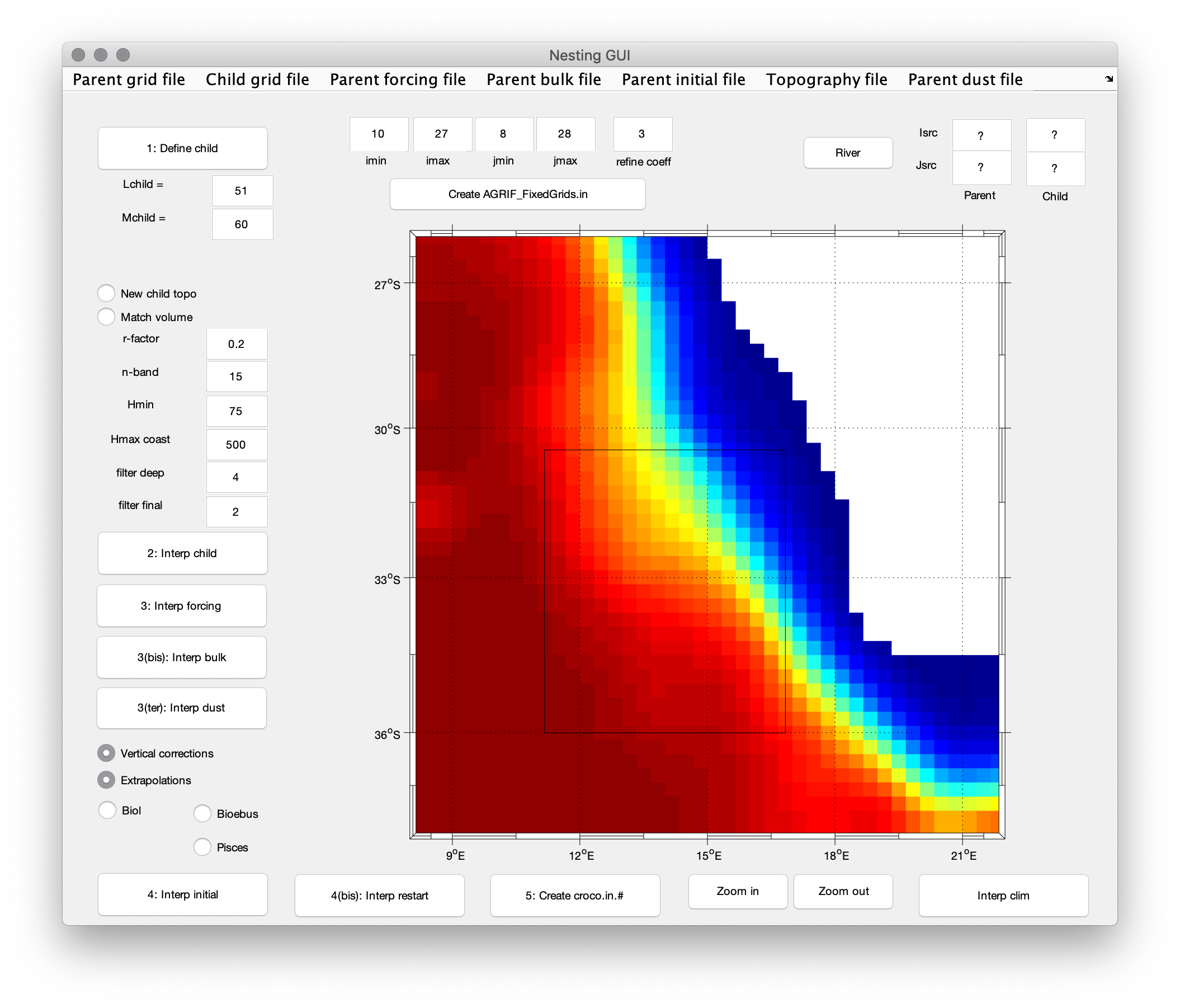

Main window of nestgui¶
Click 1. Define child and create the child domain on the main window. The size of the grid child (Lchild and Mchild) is now visible. This operation can be redone until you are satisfied with the size and the position of the child domain. The child domain can be finely tuned using the imin, imax, jmin and jmax boxes.

Warning

Be aware that the mask interpolation from the parent grid to the child grid is not optimal close to corners. Parent/Child boundaries should be placed where the mask is showing a straight coastline. A warning will be given during the interpolation procedure if this is not the case.
( If you want to change the topography input file for the child domain, click new child topo, choose your new input topo file and edit n-band which is the number of grid points on which you will connect the parent and child topography )

Click 2. Interp child to create the child grid. It generates the child grid file. Before, you should select if you are using a new topography (New child topo button) for the child grid or if you are just interpolating the parent topography on the child grid. In the first case, you should defines what topography file will be used (e.g. ~/Roms_tools/Topo/etopo2.nc or another dataset). You should also define if you want the volume of the child grid to match the volume of the parent close to the parent/child boundaries (Match volume button, it should be “on” by default). You should also define the r-factor (Beckmann and Haidvogel, 1993) for topography smoothing (“r-factor”, 0.25 is safe) and the number of points to connect the child topography to the parent topography (n-band, it follows the relation hnew = \(\alpha\). hnew + (1 - \(\alpha\)).hparent , where \(\alpha\) is going from 0 to 1 in “n-band” points from the parent/child boundaries). You should also select the child minimum depth (Hmin, it should be lower or equal to the parent minimum depth), the maximum depth at the coast (Hmax coast), the number of selective hanning filter passes for the deep regions (n filter deep” and the number of final hanning filter passes (n filter final).
Click 3. Interp forcing or 3. Interp bulk to interpolate the forcing or bulk file on the child grid. It interpolates the parent surface forcing on the child grid. Select the parent forcing file to be interpolated (e.g. Run_BENGUELA_LR/CROCO_FILES/croco_frc.nc). The child forcing file croco_frc.nc.1 will be created. The parent surface fluxes are interpolated on the child grid. You can use Interp bulk if you are using a bulk formula. In this case, the parent bulk file (e.g. Run_BENGUELA_LR/CROCO_FILES/croco_blk.nc) will be interpolated on the child grid.

( If you have changed the topography, Click Vertical interpolations)
Click 4. Interp initial or Interp restart to create initial or restart file. It interpolates parent initial conditions on the child grid. Select the parent initial file (e.g. Run_BENGUELA_LR/CROCO_FILES/croco_ini.nc). The child initial file croco_ini.nc.1 will be created. If the topographies are different between the parent and the child grids, the child initial conditions are vertically re-interpolated. In this case you should check if the options vertical corrections and extrapolations are selected. It is preferable to always use these options. If there are parent biological fields in the initial files, they can be processed automatically, we have to define the type of biological models: either NChlPZD or N2ChlPZD2, then click on the Biol button, either BioEBUS, then click on the Bioebus, either PISCES biogeochemical model, then click on the Pisces button. The fields needed for the initialization of these biological model will be processed. For information, in the case of NPZD-type (NChlPZD or N2ChlPZD2) model, there are 5 additional fields, in the case of BIOEBUS, there are 8 additional fields and in the case of PISCES biogeochemical model, there is 8 more fields.
Click 5. Create croco.in to create croco.in file for child domain
Click Create AGRIF_FixedGrids.in to create input file for AGRIF

Note

Interp clim button can be used to create a climatology file (i.e. boundary conditions) for the child to domain, to test the child domain alone or to compare 1-way online nested run and offline nested run.

This will create:

CROCO_FILES/croco_grd.nc.1
CROCO_FILES/croco_frc.nc.1  (or croco_blk.nc.1)
CROCO_FILES/croco_ini.nc.1
croco.in.1
AGRIF_FixedGrids.in

Once the input files had been build, you need to compile the model in nesting mode. You need to define AGRIF in cppdefs.h and re-compile.
You will then be able to launch croco as usual. It will run as an individual binary, with an internal loop on the number of grids. The child grid will use the *.1 files, this suffix will also be added to the output file of the nest. You can also define more than one child grid.
qsub job_croco_mpi.pbs